Design of Ground Heat Collectors: Calculation Methodology

nPro can be used to design and calculate horizontal ground heat collectors. The analytical model covers regeneration via the ground surface, ice formation around the collector pipes and the hydraulics of the collector circuits. On this page, you will learn which calculation approaches are used and which input values are reasonable. The comparison with the design values of VDI 4640 Part 2 is documented on the page Validation of the ground heat collector calculation.

Validation of the calculation

The collector calculation in nPro has been checked against VDI 4640 Part 2. The results were compared with the reference case of a doctoral thesis from TU Dresden and with the design values of VDI 4640 Part 2, Table A2 for all 15 climate zones and four soil types. All scenarios, input values and results can be found on a separate page:

➜ Validation of the ground heat collector calculation in nPro

System layout: ground heat collector with heat pump

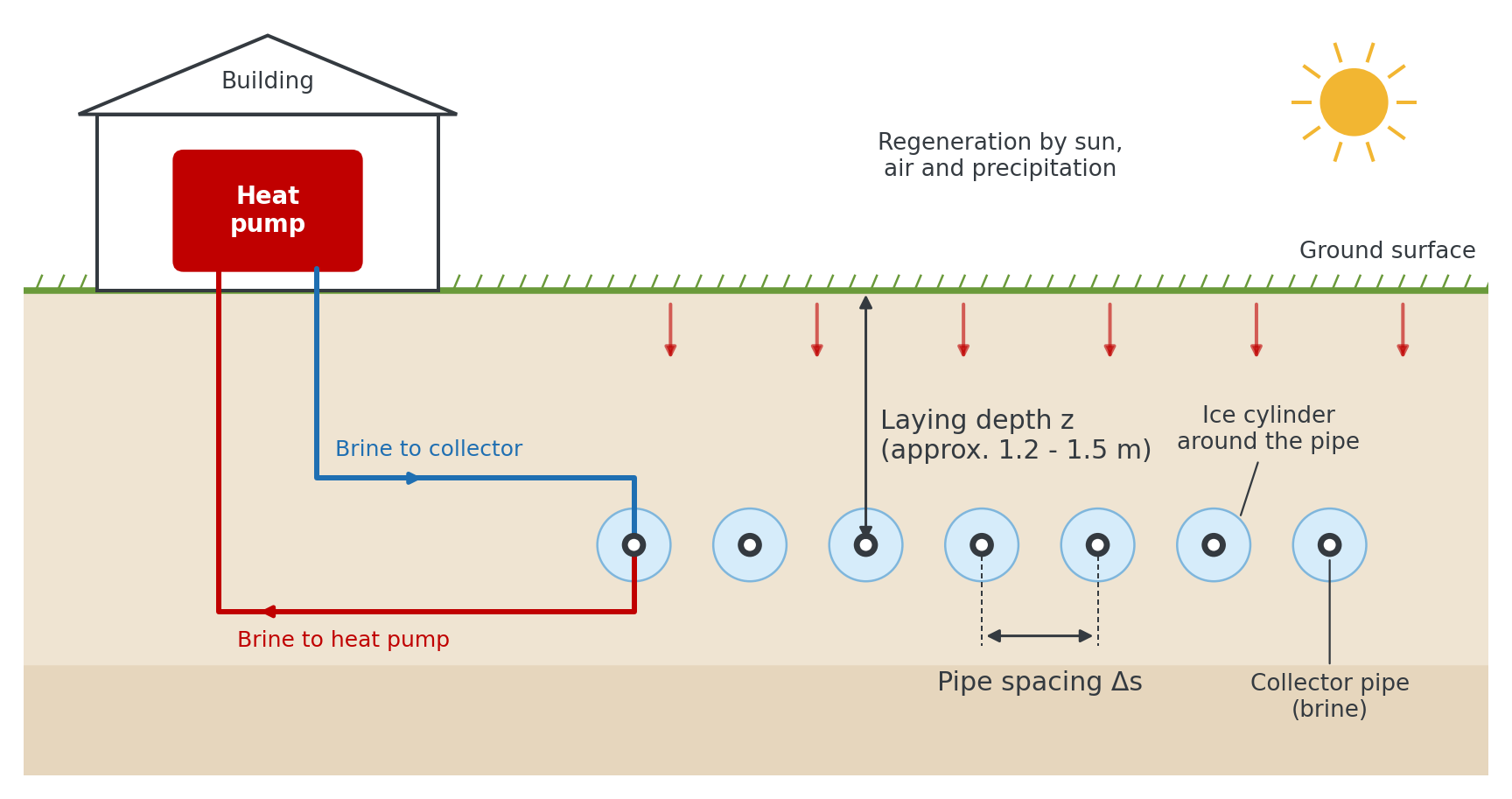
A ground heat collector consists of horizontally laid plastic pipes that are installed at shallow depth below the ground surface and through which a brine (usually a water-glycol mixture) flows. The brine absorbs heat from the surrounding soil and transfers it to the evaporator of a heat pump. The heat pump supplies either a single building or, via a heating network, an entire district.

Unlike borehole heat exchangers, collectors do not use heat from great depths but mainly solar energy stored during the summer. The soil regenerates every year via the ground surface through solar radiation, air temperature and precipitation. The key design parameters are the installation depth (z), the pipe spacing (Δs) between adjacent pipes, the pipe size and the collector area, which together with the pipe spacing determines the total pipe length.

Layout of a ground heat collector — Figure 1: Layout of a horizontal ground heat collector with heat pump: installation depth z, pipe spacing Δs and ice cylinders around the collector pipes

Fundamentals of the collector calculation

The calculation model in nPro combines an exact analytical solution of heat conduction in the soil with an ice formation model from a scientific study at TU Dresden. According to the guideline, the design values of VDI 4640 Part 2 for ground heat collectors are the result of numerical optimizations based on this study.

Three physical effects determine the performance of a collector:

Heat conduction and regeneration: The collector extracts heat from the soil, which is replenished from the ground surface and from deeper layers. Since the ground surface regenerates the soil every year, a steady periodic state is reached after one to two years. Long-term cooling of the ground over decades, as with borehole fields, does not occur.
Ice formation: If the temperature at the pipe wall drops below 0 °C, the soil water around the pipe freezes. The latent heat released in the process is a major part of the heat source. Without it, a collector could extract only about half as much heat.
Heat transfer inside the pipe: Whether the brine flow is laminar or turbulent affects the brine temperature by several kelvin. nPro therefore also calculates the hydraulics of the collector circuits.

Unlike the original calculation method of this study, nPro does not use simplified approximations for the heat flowing in from above and below, but solves the heat conduction problem of a row of pipes below the ground surface exactly for each frequency of the hourly load profile. As a result, the entire load history is taken into account, and base load, annual cycle and short-term load peaks are superimposed with the correct time shift.

How are ground heat collectors designed with nPro?

The collector module in nPro offers two calculation functions:

Calculation of the collector area at which all design criteria are met (brine temperature, maximum ice radius, thawing of ice bridges by the start of the growing season).
Calculation of the minimum brine temperature at which the brine returns from the collector to the heat pump, and of the ice formation for a given collector area.

In both cases, the hourly brine temperatures, the ice radius over the course of the year and the hydraulics (number of circuits, Reynolds number, pressure drop) are also output. A calculation takes about one second.

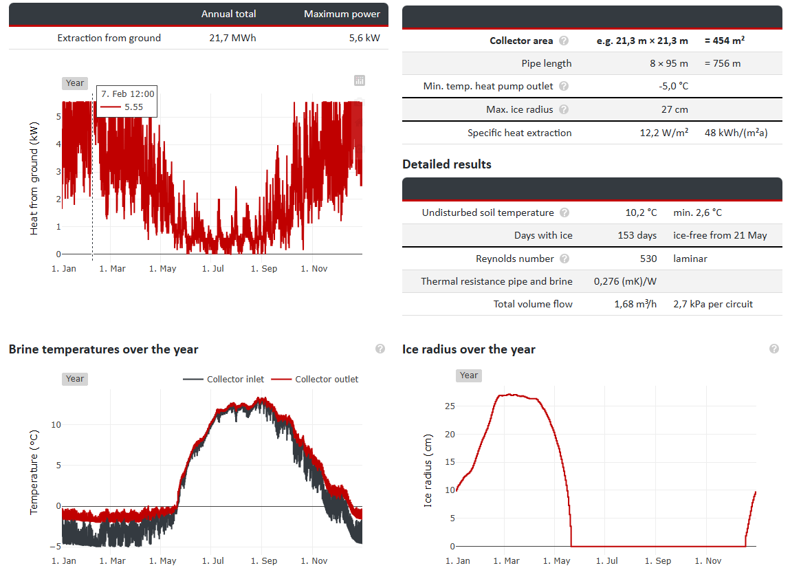
Collector design in nPro — Figure 2: Example results of the collector design in nPro: collector area, brine temperatures, ice radius and hydraulics.

For the calculation, nPro uses the hourly heat extraction profile of the heat pump calculated in the operational simulation and the hourly air temperature profile of the selected location. The collector field is assumed to be sufficiently large so that edge effects can be neglected. In reality, additional heat flows in from the sides at the edges, so this assumption is on the safe side.

Calculation methodology

Undisturbed ground temperature

The temperature of the undisturbed soil at installation depth follows the annual cycle of the air temperature, but damped and with a time lag. At a depth of 1.2 m, the temperature minimum occurs about three to four weeks after the minimum of the air temperature. nPro decomposes the hourly air temperature profile of the location into its frequency components and damps each component according to the heat conduction in the soil and the heat transfer at the ground surface (solution according to Grigull and Sandner):

Calculation basis:

\begin{gathered} T_{undisturbed}(z, \omega) = T_{air}(\omega) \cdot \frac{e^{-m z}}{1 + \lambda m / \alpha} \quad \text{with} \quad m = (1+i) \sqrt{\frac{\omega}{2a}} \end{gathered}

Here, ω is the angular frequency, a is the thermal diffusivity of the soil and α is the heat transfer coefficient at the ground surface (15 W/(m²K)). For the annual mean, e⁰ = 1 applies, i.e. the mean ground temperature equals the mean air temperature.

Heat conduction in unfrozen soil

The collector is modelled as an infinite row of parallel pipes with spacing Δs at depth z below the ground surface. For the steady-state case, the thermal resistance per metre of pipe is given in closed form:

Calculation basis:

\begin{gathered} R'_{soil} = \frac{1}{2 \pi \lambda} \ln\left( \frac{2 \Delta s}{\pi d_a} \sinh\frac{2 \pi z}{\Delta s} \right) \approx \frac{z}{\lambda \, \Delta s} + \frac{1}{2 \pi \lambda} \ln\frac{\Delta s}{\pi d_a} \end{gathered}

The approximation clearly shows the two components: the first term describes the heat conduction from the ground surface through the soil layer of thickness z, the second the convergence of the heat flow towards the individual pipe.

For the time-dependent behaviour, nPro decomposes the hourly heat extraction profile into its frequency components using a Fourier transform. For each component, the temperature response of the soil is known analytically: a planar component (heat sink in the collector plane with heat transfer at the ground surface) and a local component around the pipes (Fourier series along the row of pipes). The sum of all components yields the hourly drop in pipe wall temperature relative to the undisturbed soil.

Ice formation around the collector pipes

As soon as the pipe wall reaches 0 °C, an ice cylinder forms around the pipe. nPro then calculates in daily time steps using the following approach:

At the ice surface, the temperature is constantly 0 °C. The heat flow from the unfrozen soil to the ice surface results from the heat conduction model.
The difference between extracted heat and inflowing heat causes soil water to freeze (or to thaw in spring). This yields the cross-sectional area of the frozen soil:

\begin{gathered} A_{ice} = \frac{E_{ice}}{\theta_f \cdot \rho_w \cdot \Delta h_s} \end{gathered}

with the stored latent heat E_ice per metre of pipe, the freezable water content θ_f, the density of water ρ_w and the enthalpy of fusion Δh_s = 333.5 kJ/kg.

The pipe wall temperature results from heat conduction through the frozen soil from the ice surface to the pipe:

\begin{gathered} T_{pipe\,wall} = 0\,°C - q' \cdot \frac{\ln(r_{ice} / r_a)}{2 \pi \lambda_{frozen}} \end{gathered}

If the ice cylinders of adjacent pipes grow together, the ice can only expand upwards and downwards. The ice radius and heat conduction through the ice are then calculated with equations for merged ice cylinders.

The simulation runs over several years until the annual cycle of freezing and thawing repeats itself. Sensible heat in the frozen zone is neglected.

Calculation of brine temperatures

The brine temperatures are calculated hourly from the pipe wall temperature (or from the undisturbed ground temperature and the temperature drop in the soil), the thermal resistance of the pipe wall and brine, and the temperature spread. As in VDI 4640 Part 2, the design-relevant value is the temperature of the brine returning from the collector to the heat pump (collector outlet). The brine at the heat pump outlet (collector inlet) is colder by the temperature spread:

Calculation basis:

\begin{gathered} T_{brine \rightarrow HP}(t) = T_{pipe\,wall}(t) - q'(t) \cdot R'_{pipe} + 0.5 \, \Delta T_{fluid}(t) \\ T_{HP \rightarrow brine}(t) = T_{brine \rightarrow HP}(t) - \Delta T_{fluid}(t) \end{gathered}

The mass flow rate is assumed to be constant and is sized so that the set temperature spread is reached at maximum heat extraction. At part load, the temperature spread is correspondingly smaller.

Hydraulics of the collector circuits

The total pipe length is divided into parallel collector circuits of equal length. nPro selects the number of circuits so that the brine flow is turbulent at maximum load (Reynolds number approx. 2500, VDI 4640 Part 2: 2300 to 3000) without exceeding the set maximum circuit length. If this cannot be achieved, the maximum circuit length applies and nPro indicates that the flow is laminar. The Reynolds number, heat transfer and pressure drop are derived from the volume flow per circuit. The thermal resistance between the brine and the outer pipe wall consists of heat conduction through the pipe wall and convective heat transfer:

Calculation basis:

\begin{gathered} R'_{pipe} = \frac{\ln(d_a / d_i)}{2 \pi \lambda_{pipe}} + \frac{1}{\pi \, d_i \, h} \end{gathered}

The heat transfer coefficient h is calculated with a constant Nusselt number for laminar flow and according to Gnielinski for turbulent flow. The fluid properties of the brine correspond to a propylene glycol-water mixture (25 %) at 0 °C. Laminar flow more than doubles the pipe resistance. VDI 4640 Part 2 therefore recommends a Reynolds number between 2300 and 3000.

Design criteria

When calculating the collector area, nPro searches for the smallest area at which all of the following criteria are met:

Minimum brine temperature: The temperature of the brine returning to the heat pump does not fall below the set limit in any hour (VDI 4640 Part 2: -5 °C).
Maximum ice radius: The frozen zone around a pipe does not extend vertically beyond the limit (recommendation from the literature: 0.5 m).
Ice bridges thawed by the start of the growing season: Merged ice cylinders must have thawed as soon as the monthly mean air temperature exceeds 12 °C. This allows rainwater and meltwater to seep away and does not impair plant growth above the collector. The values in VDI 4640 Part 2, Table A2 are based on this criterion.
Maximum brine temperature in cooling mode: If the collector is also used for cooling, the temperature at the collector outlet does not exceed the limit.

In addition, nPro indicates if the annual heat extraction exceeds 70 kWh/(m²a) or if the flow in the collector circuits is laminar.

Assumptions and limitations of the model

The results apply to the steady periodic year. The heat extraction profile is assumed to repeat every year.
All temperatures are hourly mean values. On/off cycling of the heat pump is not modelled. For heat pumps in on/off operation, the brine temperature during operating periods is about 1 to 3 K lower than the hourly mean.
The mean ground temperature is set equal to the mean air temperature. In measurements, it is usually more than 1 K higher, so this assumption is on the safe side.
Edge effects of the collector field are neglected (safe side).
Regeneration and cooling are taken into account: hours with heat injection into the soil (e.g. cooling or solar thermal) are included in the calculation with their entire load history and melt any existing ice. Because the collector is installed at shallow depth, heat injected in summer largely dissipates via the ground surface by winter; regeneration during the heating season has a significantly greater effect.
Drying out of the soil at high injection temperatures, which reduces thermal conductivity, is not modelled. The maximum temperature at the collector outlet in cooling mode should therefore be chosen conservatively.
An insulating snow cover is not taken into account. In very cold climate zones, where the soil at installation depth freezes even without heat extraction, the results are therefore very conservative; nPro indicates this in such cases.
Compact designs such as geothermal baskets, trench collectors or spiral collectors are not part of the model.

Validated value ranges and determination of input values

This section explains which guide values can be used for the input parameters of the collector calculation.

Table 1: Typical value ranges of the input parameters and possible sources for determining suitable input values.

Parameter	Typical range	Data source
Installation depth	1.2 - 1.5 m, at least 30 cm below frost depth	VDI guideline 4640 Part 2
Pipe spacing	0.2 - 0.75 m, depending on soil and climate zone	VDI guideline 4640 Part 2, Table A2
Collector pipe	PE 32 × 3.0 mm (reference of the VDI tables), also 25 × 2.3 mm or 20 × 2.0 mm	Manufacturer data
Max. length per circuit	approx. 200 - 300 m for PE 32 so that turbulent flow is achieved; check pressure drop	VDI guideline 4640 Part 2, manufacturer data
Temperature spread	approx. 3 K	Heat pump manufacturer data
Min. temp. of brine to heat pump	-5 °C	VDI guideline 4640 Part 2, heat pump manufacturer data
Max. ice radius	0.5 m	Scientific literature (TU Dresden)
Soil parameters	see soil types below	Geotechnical report, VDI guideline 4640 Parts 1 and 2

Soil types and soil parameters

The performance of a collector depends strongly on the water content of the soil. It determines the thermal conductivity, the heat capacity and, above all, the latent heat released during freezing. nPro offers four soil types according to VDI 4640 Part 2. Thermal conductivity and water content correspond to Table A1 of VDI 4640 Part 2. Heat capacity and thermal conductivity in the frozen state are taken from soil tables in the scientific literature. The freezable water content is the water content minus the fraction that remains unfrozen at about -2 °C.

Table 2: Soil parameters of the soil types available in nPro (VDI 4640 Part 2, Table A1, supplemented by literature values).

Soil type	Water content in vol.%	Thermal conductivity in W/(mK)	Heat capacity in MJ/(m³K)	Thermal conductivity frozen in W/(mK)	Freezable water content in m³/m³
Sand	< 10	1.2	1.2	1.4	0.08
Loam	25 - 31	1.5	2.2	2.4	0.25
Silt	35 - 40	1.5	2.4	2.6	0.35
Sandy clay	35 - 40	1.8	2.4	2.9	0.29

With the User-defined option, all soil parameters can be entered freely, for example based on a geotechnical report. According to VDI 4640 Part 2, in water-saturated soils the collector can be designed as for sandy clay, regardless of the actual soil type. A freezable water content of 0 disables ice formation in the model.

Sources

VDI guideline 4640 Part 2: “Thermal use of the underground - Ground source heat pump systems”. Verein Deutscher Ingenieure, 2019.
VDI guideline 4640 Part 1: “Thermal use of the underground - Fundamentals, approvals, environmental aspects”. Verein Deutscher Ingenieure.
Grigull, U.; Sandner, H.: “Wärmeleitung” (Heat Conduction). Springer-Verlag, 2nd edition, 1990.
Gnielinski, V.: “Neue Gleichungen für den Wärme- und den Stoffübergang in turbulent durchströmten Rohren und Kanälen” (New equations for heat and mass transfer in turbulent pipe and channel flow). Forschung im Ingenieurwesen 41 (1975), pp. 8-16.
pygfunction code repository by Massimo Cimmino (brine properties and heat transfer inside the pipe)