

In this case study, a district with heating and cooling demands is supplied via a cold district heating network. The entire planning process can be carried out in the nPro tool: from the demand calculation through the pipe dimensioning and the design of the heat and cold generators to the economic feasibility calculation. The heat sources are a sewage heat source and a borehole field that is fully regenerated.
Initial situation and project setup
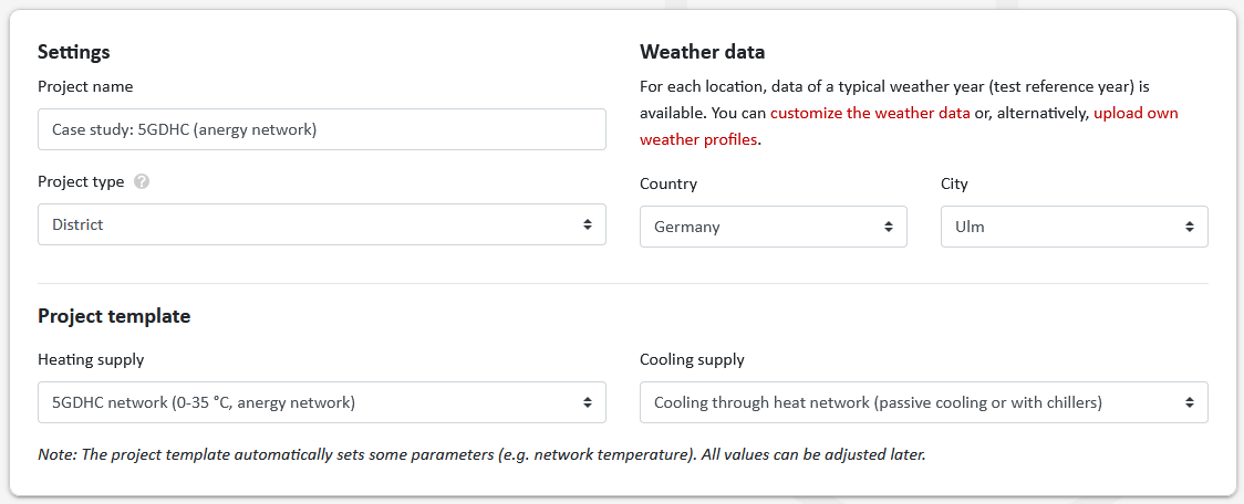
The supply area is a mixed-use district in Ulm: 36 buildings that are supplied with both heating and cooling via a cold district heating network (anergy network). For this location, nPro provides the data of a typical weather year (test reference year); alternatively, your own weather data can be uploaded.
When creating the project, the project type district is selected and, as the project template, the combination of a cold district heating network (0–35 °C) and cooling via the heating network. The template presets a number of parameters to match the network type, the network temperatures for example, and all values remain freely adjustable afterwards.
The supply area
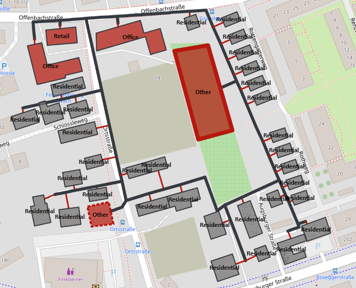
The district brings exactly the mix of uses for which an anergy network is suited. In the residential buildings, decentralized booster heat pumps use the network as a heat source and thereby cover space heating and domestic hot water. Two office buildings are additionally air-conditioned and feed their waste heat into the network. In addition, there is a retail building that requires process cooling alongside air conditioning. This cooling demand arises all year round and therefore also delivers waste heat in winter.
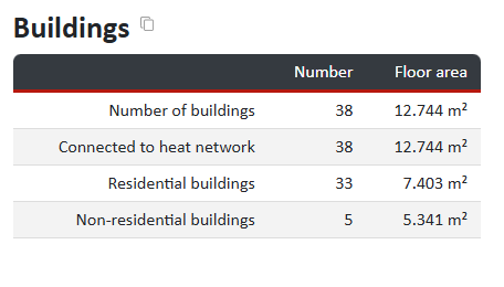
In total, 36 buildings with 12,744 m² of floor area are connected to the network, including 33 residential buildings with 7,403 m². In addition, there are two plots for the energy centers, which have no demand of their own and are listed in the building overview.
Parameters of the heating network
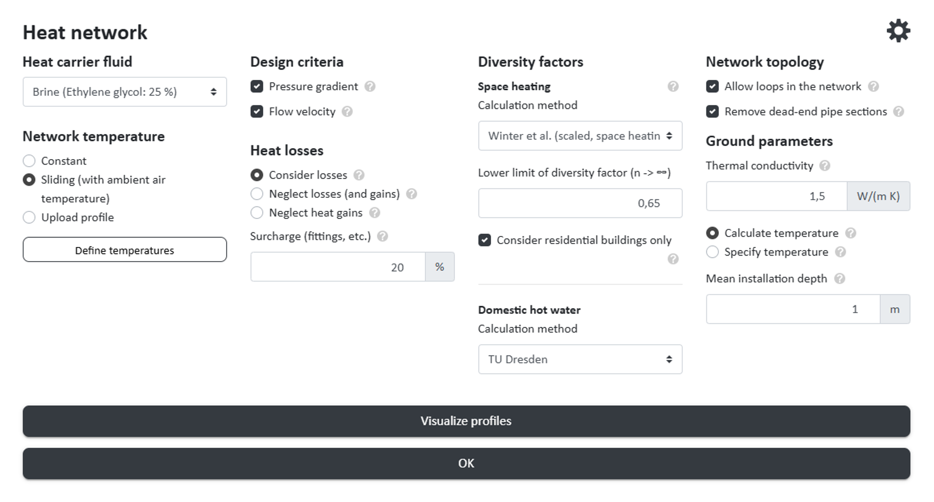
The network is parameterized in detail in nPro. The heat transfer fluid in this case example is brine with a 25 % ethylene glycol content, and the network temperature follows a sliding curve as a function of the outside air temperature. The heat losses are taken into account, supplemented by a surcharge of 20 % for valves and fittings. In an anergy network, the network also absorbs heat from the ground along the way. The dimensioning follows the design criteria of pressure gradient and flow velocity.
The simultaneity factors follow the approach by Winter et al. with a lower limit of 0.65 for space heating and the approach of TU Dresden for domestic hot water. In the network topology, meshes are permitted and free pipe ends are removed automatically. For the ground, a thermal conductivity of 1.5 W/(m K) at a mean burial depth of 1 m is applied, and the ground temperature is calculated.
The network temperatures are defined via two support points: 8/5 °C at −10 °C outside air temperature and 12/9 °C at +2 °C. The network therefore behaves exactly the opposite way to a conventional heating network: in winter it is colder, because a lot of heat is extracted from the heat source, and in summer it is warmer. The temperature spread of 3 K is maintained across the entire curve.
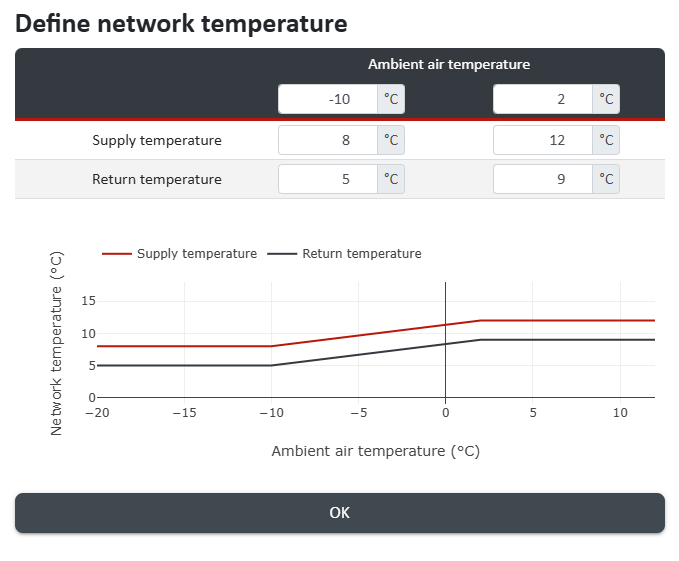
On this basis, nPro calculates the pipe dimensioning, the network temperatures, the heat losses and the pumping work. The results are presented in the following section.
Results of the network simulation
Units in the buildings
From the demand profiles and the network temperatures, nPro dimensions the units in every building. In the district, this results in 36 booster heat pumps with a combined 619 kWth, which provide 1,215 MWh of useful energy with an electricity demand of 252 MWh. This corresponds to a seasonal performance factor of 4.8. In addition, there are 36 heat transfer stations with 528 kWth and domestic hot water storage tanks with a total of 10,800 l.
On the cooling side, the strength of the cold network becomes apparent: for the entire cooling demand of the district, only one network chiller with 7.8 kWth is required. The remaining cooling demand is covered passively via heat exchangers from the network, entirely without a chiller.

Pipe dimensioning
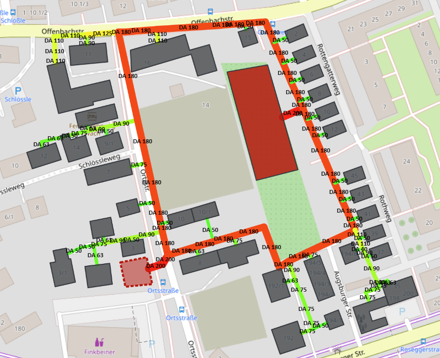
nPro determines the nominal diameter for every network section. The nominal diameters range from DA40 in the house connections to DA200 at the two feed-in points.
The network contains a mesh: the ring connects the two energy centers in the north-east and on Ortsstraße with one another. In meshed sections, the flow direction is no longer unique, because it depends on the respective load case. nPro therefore dimensions these sections uniformly for the most unfavorable case. This becomes visible in the continuous DA180 along the ring.
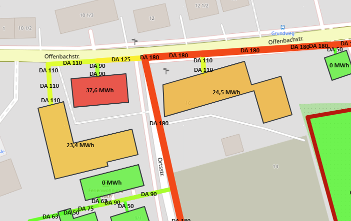
Besides the nominal diameters, the energy amounts of the buildings can also be displayed on the map, for example the waste heat fed into the network. In the north-west of the district, this immediately shows which buildings act as heat suppliers: the retail and office buildings feed in between 23.4 and 37.6 MWh of waste heat from the cooling supply, while the residential buildings only draw heat.
Network properties, pumping work and pressure
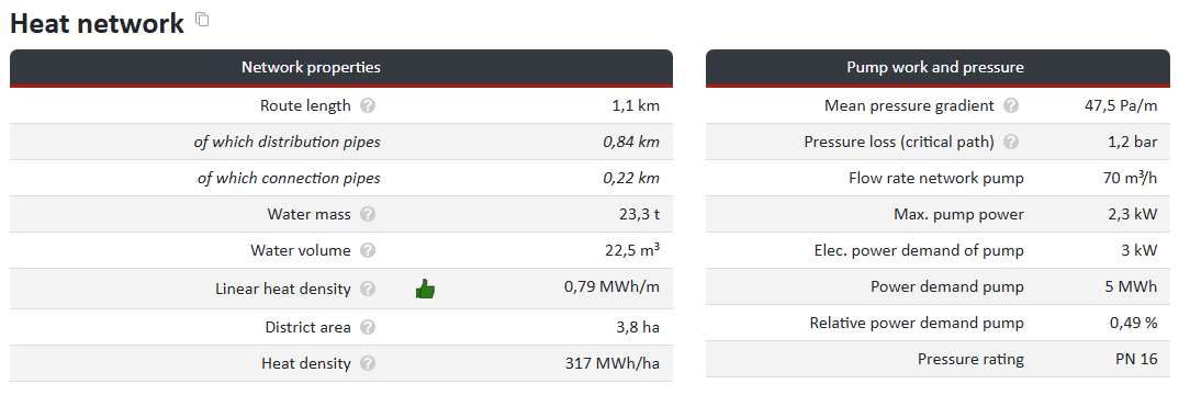
The network is 1.1 km long, of which 0.84 km are distribution lines and 0.22 km house connections. At 1,215 MWh of heating demand, this results in a linear heat density of 0.79 MWh/m and a heat density of 317 MWh/ha across 3.8 ha of district area.
The pumping work is remarkable: at 5 MWh, it corresponds to only 0.49 % of the electricity demand in the district. The frequently cited argument against cold networks, namely a high pumping effort due to the small temperature spread, does not carry weight in this example. The volume flow of the network pump is 70 m³/h and the maximum pumping capacity 2.3 kW.
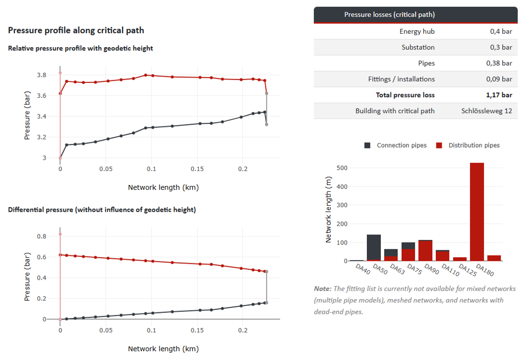
The pressure loss to the critical point of the network amounts to 1.17 bar in total and is distributed across the energy center, the heat transfer station, the pipes and the pipe fittings. Besides the pressure profile, optionally with or without the influence of the geodetic height, nPro also outputs the distribution of the nominal diameters over the network length, separated into distribution lines and house connections.
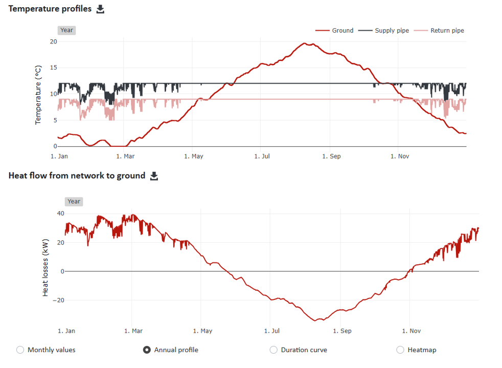
The temperature profiles show the relationship that characterizes an anergy network: supply and return lie between 5 and 12 °C all year round, while the ground temperature at a depth of 1 m fluctuates seasonally between 0 and 20 °C. In winter, the network therefore releases heat to the ground, and in summer it absorbs heat. Over the year, this adds up to 105 MWh of heat losses and 31 MWh of heat gains.
Heating, cooling and electricity use
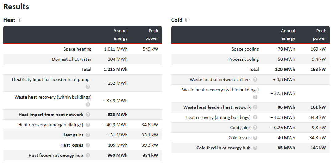
The results overview converts the demands of the buildings step by step into the load at the energy center. 1,215 MWh of heating demand become 960 MWh of heat feed-in at the energy center:
First, the booster heat pumps cover 252 MWh from electricity, and a further 37.3 MWh comes from heat recovery within the buildings. The heat drawn from the network thus falls to 926 MWh. Within the network, 40.3 MWh of heat recovery between buildings and 31 MWh of heat gains are added, while 105 MWh occur as heat losses. The maximum capacity is reduced from a 549 kW heating load to 384 kW at the energy center.
On the cooling side, the calculation runs in parallel: of 120 MWh of cooling demand, 86 MWh are fed into the network as waste heat, 40.3 MWh of which are reused directly between the buildings. At the energy center, 85 MWh of cooling feed-in remain, that is, the same waste heat that the network simultaneously uses as a heat source.
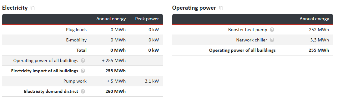
The electricity demand of the district amounts to 260 MWh, of which 252 MWh are for the booster heat pumps, 3.3 MWh for the network chiller and 5 MWh for pumping work. User electricity and electric mobility are not taken into account in this case example.
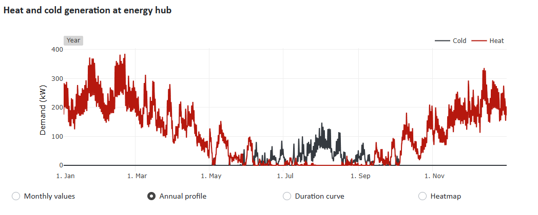
The annual profile of the feed-in at the energy center shows the seasonal division of labor: from November to April, heat dominates with peaks of around 380 kW; in July and August the picture reverses and cooling takes over. In the transitional months, both loads occur simultaneously. This is precisely the situation in which heating and cooling demand partly balance each other within the network.
Energy supply system
Generator structure
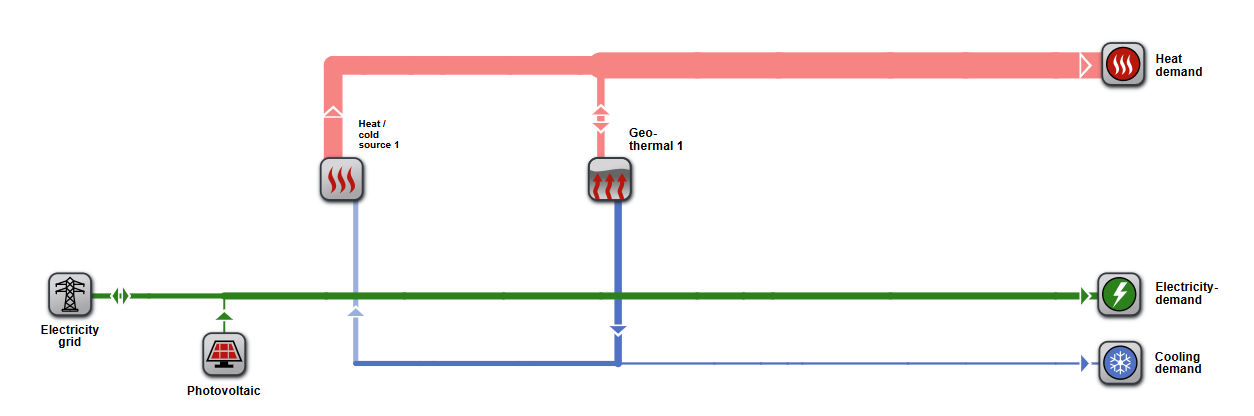
The heat and cooling supply at the energy center is provided by two sources that complement each other seasonally: a sewage heat source, set up in nPro as Heat Source 1, which feeds low-temperature heat into the network via a heat exchanger, and a borehole field, set up as Geothermal probe 1, which both delivers heat and provides cooling while being regenerated in the process. The system is supplemented by a photovoltaic system whose area is determined by the optimization and which covers part of the operating electricity of the booster heat pumps directly within the district.
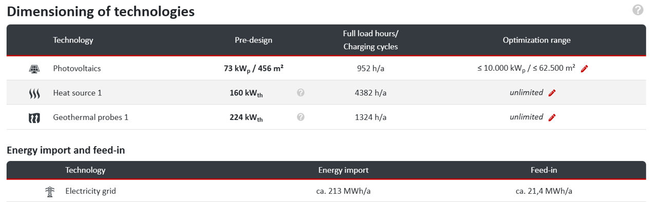
Which technologies are built with which capacity is determined by the design optimization in nPro on the basis of the investment and operating costs. The division of roles between the two sources results from the calculation itself and does not have to be specified. It turns out clearly: Heat Source 1 covers the base load with 160 kWth and 4,382 full-load hours, while Geothermal probe 1 complements it with 224 kWth and 1,324 full-load hours. The optimization sizes the photovoltaic system at 73 kWp on 456 m².
Of the district’s electricity demand, around 213 MWh therefore remain as grid purchase, while 21.4 MWh are fed into the electricity grid.
Heat Source 1: sewage heat
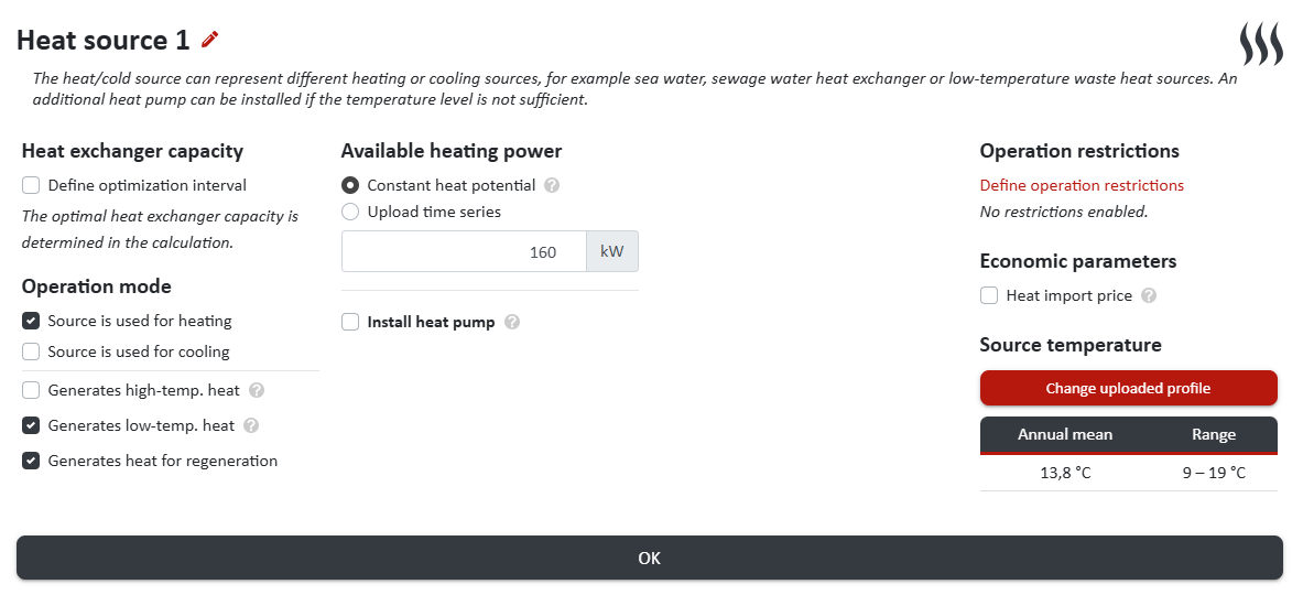
The sewage heat is represented by the Heat Source 1 module and applied with a constant heat potential of 160 kW. An annual profile is entered for the source temperature: it ranges between 9 and 19 °C with an annual mean of 13.8 °C, at the lower end in winter, when the heat is needed, and at the upper end in summer.
Because the temperature level lies above the network temperature all year round, no additional heat pump is required; the source feeds in directly via the heat exchanger. The capacity of the heat exchanger is determined by the optimization calculation.
Two operating modes are active: the source is used for heating and generates heat for the regeneration of the borehole field. It therefore not only contributes to the heat supply but also charges the ground in summer.
Geothermal probe 1: borehole field
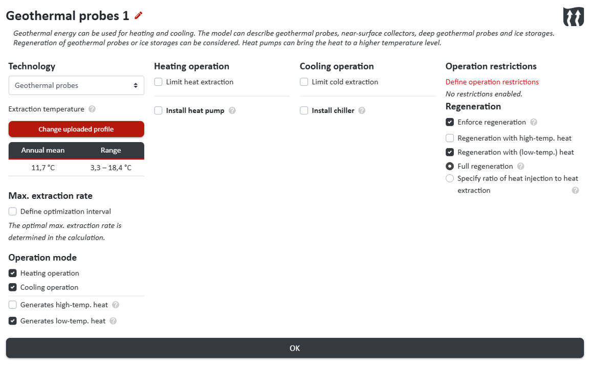
The borehole field is represented by the Geothermal probe 1 module with the technology probes and used both in heating operation and in cooling operation. The latter is the basis of the passive cooling in the district. The extraction temperature is available as a profile, with an annual mean of 11.7 °C and a value range of 3.3 to 18.4 °C.
Decisive for the design is the specification regarding regeneration: “force regeneration” and “complete regeneration” with low-temperature heat are activated. Over the year, exactly as much heat is therefore returned to the ground as was extracted from it. As a result, the borehole field does not work as a permanent heat source but as a seasonal storage, charged from sewage heat and the waste heat of the cooling supply.
Energy flow diagram
After the operational simulation, nPro displays the energy flows of the overall system. The thickness of the lines is proportional to the amount of energy transferred; the values are shown when hovering over them with the mouse pointer.
The dual role of the borehole field is clearly visible: from the geothermal system, one line leads to the heating demand and another to the cooling demand. Heat Source 1 feeds in exclusively on the heating side, while the photovoltaic system feeds into the district’s electricity grid and thereby helps cover the operating electricity of the heat pumps.
Design of the boreholes
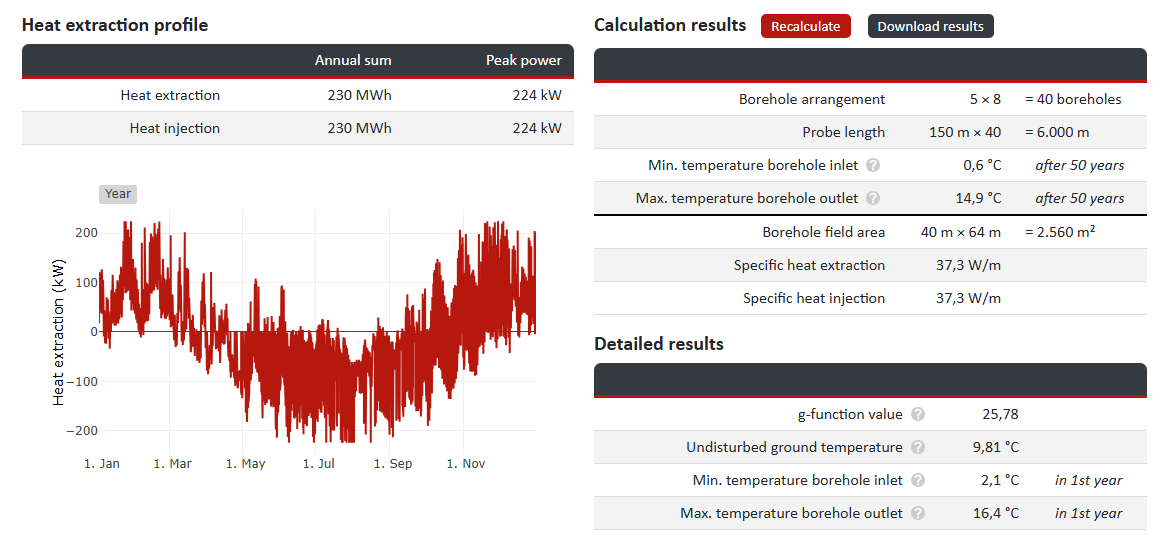
On the basis of the simulated extraction profile, nPro designs the borehole field in detail. The result is 40 boreholes with a length of 150 m each, i.e. 6,000 borehole meters on a borehole field area of 2,560 m². The specific heat extraction amounts to 37.3 W/m and thus lies within the usual design range.
Heat extraction and heat injection are exactly equal at 230 MWh and 224 kW each. This is not a coincidence but a consequence of the enforced regeneration.
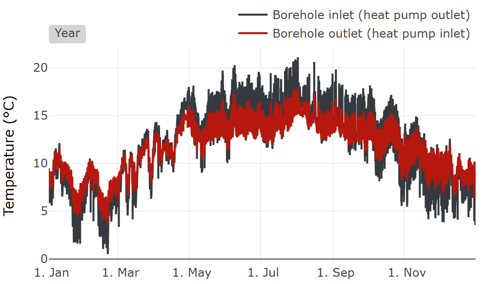
The effect becomes apparent in the temperatures: at the borehole inlet, the minimum is 2.1 °C in the first year and 0.6 °C after 50 years; at the borehole outlet, the values are 16.4 and 14.9 °C respectively. Over half a century of operation, the temperatures therefore drift by only about 1.5 K. With a balanced heat budget, the ground does not cool down.
The simulation also provides the annual profile of the fluid temperatures at the borehole inlet and outlet. It follows the seasonal operating mode of the storage: in winter, the temperatures fall to about 1 °C; in summer, they rise above 20 °C during charging.
Heat generation and regeneration
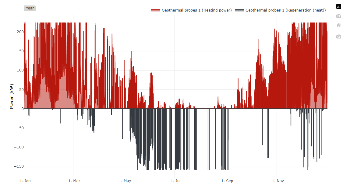
How the borehole field is operated over the year is made visible by the operational simulation. From November to April, heat generation predominates with capacities of up to 224 kW. From May to September, operation reverses: regeneration then dominates, with injection capacities of up to about 160 kW.
During the transitional periods, both operating modes alternate within a few hours: the field delivers heat in the morning and is recharged from cooling waste heat around midday. It is precisely this hourly resolution that is needed to close the balance over the year.
Economic feasibility
Finally, nPro assesses the energy system economically, using the net present value and annuity method based on VDI 2067, including replacement investments and residual values. A period under consideration of 20 years and a discount rate of 5 % are applied.
Key figures
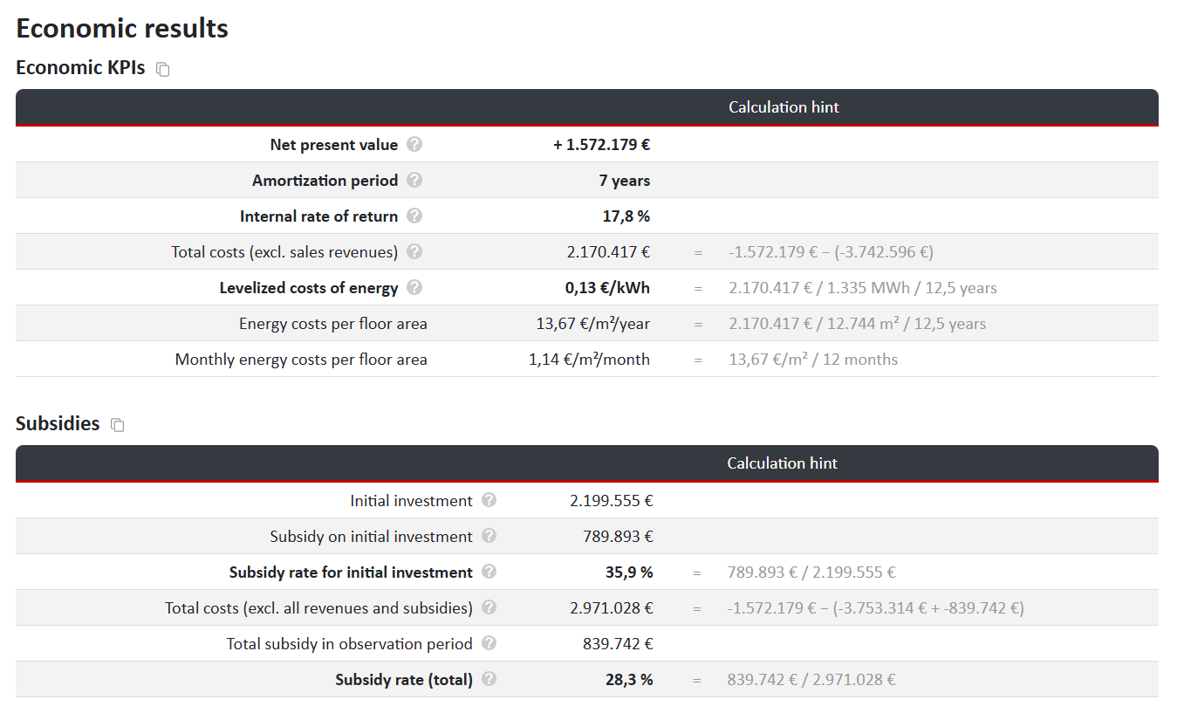
The project is viable under the assumptions made: the net present value after 20 years is +1,572,179 €, the payback period is 7 years and the internal rate of return 17.8 %, considerably above the applied discount rate of 5 %. The levelized cost of energy amounts to 0.13 €/kWh, which in relation to the floor area corresponds to 13.67 €/m² per year or 1.14 €/m² per month.
In nPro, every key figure carries a calculation note that discloses the underlying calculation. The figures therefore do not stand on their own but remain traceable down to the input variables.
The subsidies are reported separately: of the initial investment of 2,199,555 €, 789,893 € are covered by subsidies, i.e. a subsidy rate of 35.9 %. Over the entire time horizon considered, including the operating cost subsidy, the subsidies add up to 839,742 €, corresponding to an overall subsidy rate of 28.3 %.
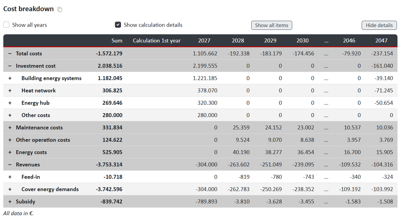
Cost breakdown
The cost breakdown itemizes all positions over the period under consideration. The investment costs of 2,038,516 € are distributed across the building energy systems (1,182,045 €), the heating network (306,825 €), the energy center (269,646 €) and other costs (280,000 €).
The distribution is typical for a cold network: the largest block is not accounted for by the trench but by the decentralized units in the buildings, that is, the 36 booster heat pumps together with transfer stations and storage tanks. The network itself accounts for only around 15 % of the investment.
On the cost side, energy costs (525,905 €), maintenance costs (331,834 €) and other operating costs (124,622 €) are added. These are offset by revenues of 3,753,314 €, which stem almost entirely from covering the energy demands, as well as the subsidy of 839,742 €.
Using the buttons, the calculation details of the first year can be displayed, the table extended by one column per year and the hierarchy expanded down to the individual unit.
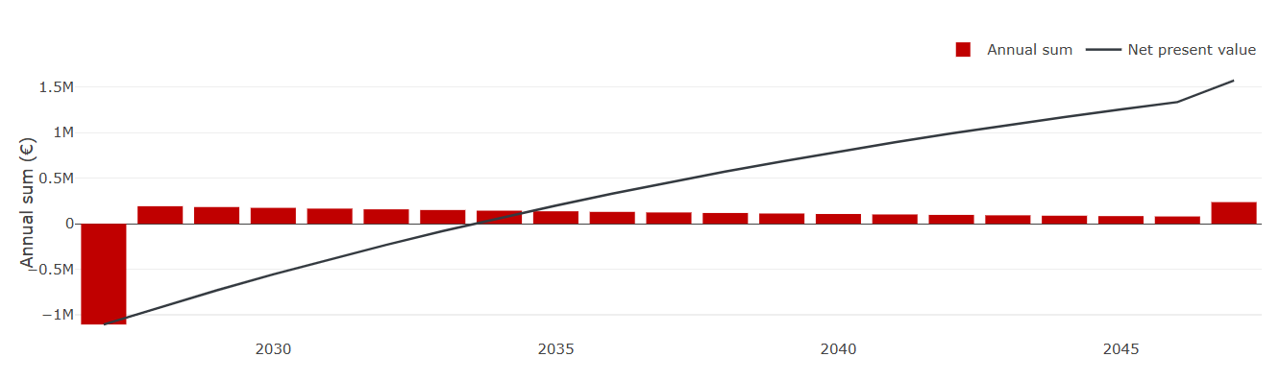
Net present value curve
The curve shows the annual totals as bars and the cumulative net present value as a line. In the first year, the initial investment weighs in negatively with a good one million euros, already reduced by the subsidy, which is granted in the same year. Afterwards, the system generates annual surpluses, and the net present value becomes positive after 7 years.
The higher bar in the final year contains the residual values of those units whose technical service life extends beyond the time horizon considered, above all the heating network and the boreholes.
Video tutorial on cold district heating
You can find a detailed video tutorial on calculating cold district heating networks here:
