

On this page you will learn how nPro models air-source heat pumps: from the nominal electrical capacity and the sectors and temperatures to the calculation of the COP from product data or via the Carnot approach. We also show which values to take from a manufacturer’s data sheet and how to account for the output plateau of air-source heat pumps at high outdoor temperatures via a limit temperature.
Operating principle
An air-source heat pump extracts heat from the outdoor air in the evaporator. Using electricity, the compressor raises this heat to a higher temperature level, and the condenser transfers it to the heating circuit. The ratio of heat delivered to electricity consumed is the COP (coefficient of performance).
The COP depends mainly on the temperature lift between the heat source (outdoor air) and the heat sink (flow temperature): the smaller the lift, the higher the COP. Since the outdoor temperature varies over the year, the COP of an air-source heat pump changes from hour to hour. For heat pumps with a speed-controlled compressor (inverter), it also depends on the load: they usually work most efficiently at medium speed and less efficiently at maximum speed.
In cooling mode, the heat pump works the other way round: it extracts heat from the cooling circuit and releases it to the outdoor air. The efficiency in cooling mode is described by the EER (energy efficiency ratio), the ratio of cooling output to electricity consumed. Since the heat released to the outdoor air equals the sum of cooling output and electricity, EER = COP − 1 applies.
Modelling in nPro
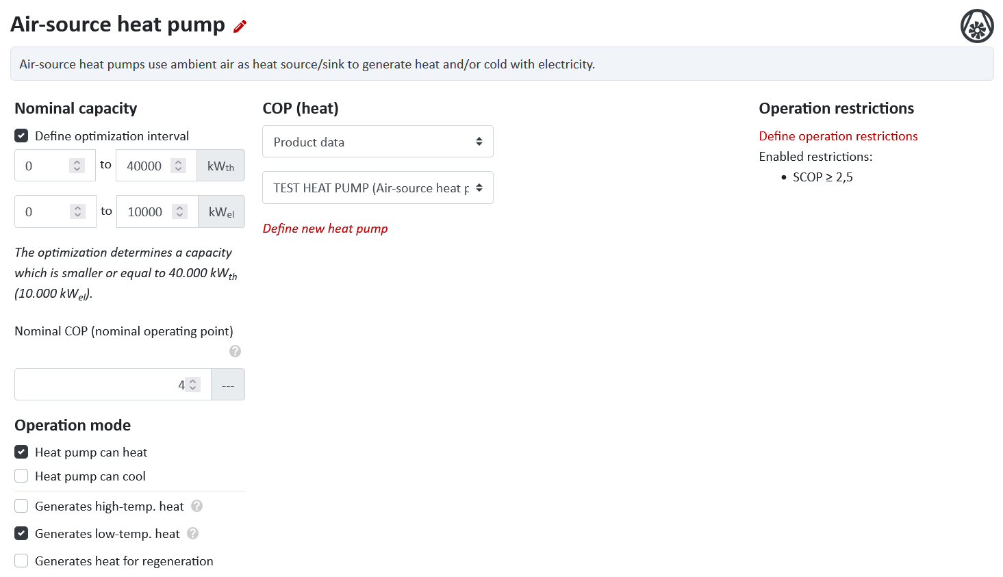
Nominal electrical capacity and nominal COP
In nPro, the actual capacity of the air-source heat pump is its nominal electrical capacity, i.e. its maximum electricity consumption. It is the same in all hours. The maximum heat output in an hour is the product of the nominal electrical capacity and the COP of that hour:
You specify the optimization range in kWth or kWel. Both values are linked via the nominal COP, the COP at the rated operating point of the heat pump. If the lower and upper bounds are equal, the capacity is fixed and not optimized. The nominal COP is only used for this conversion and has no influence on the hourly efficiency.
The displayed nominal thermal capacity is therefore the heat output at the nominal COP. In hours with a lower COP, the heat pump delivers less heat. An example: with a nominal COP of 4, 68 kWel correspond to a nominal thermal capacity of 272 kWth. In a cold hour with a COP of 2.3, however, the same heat pump can only deliver 156 kW.
Operating modes and sectors
Under Operating mode, you define whether the heat pump can heat, cool or both. In heating mode, it can serve three sectors:
- Low-temperature heat: the standard sector for heat supply, as long as several temperature levels do not have to be represented explicitly. In the energy flow diagram, the connections are light red.
- High-temperature heat: for projects in which several temperature levels are represented explicitly. In the energy flow diagram, the connections are dark red.
- Heat for regeneration: heat at the temperature level of the cooling side, for example for the regeneration of boreholes or of a 5GDHC network. In the energy flow diagram, the connections are light blue.
For each sector, the COP results from the outdoor air as heat source and the temperature of the respective demand as heat sink:
| Sector | Heat source | Heat sink (building, energy hub) | Heat sink (district) |
|---|---|---|---|
| Low-temperature heat | Outdoor air | LT flow temperature: constant, sliding or uploaded | Threshold temperature between HT and LT, if defined, otherwise network supply |
| High-temperature heat | Outdoor air | HT flow temperature: constant, sliding or uploaded | Network supply |
| Regeneration | Outdoor air | Cooling demand temperature | Network return or 6 °C with a separate cooling network |
| Cooling | Cooling demand temperature | Outdoor air | Network return or 6 °C with a separate cooling network |
A sliding flow temperature is calculated from the outdoor temperature either linearly between two support points or via a heating curve and is limited to 20 to 90 °C.
All sectors share the nominal electrical capacity. How the capacity is distributed among the sectors in each hour is decided by the optimization model.
COP calculation
For each sector, you choose how the COP is determined:
- Constant value: a fixed COP for all hours.
- Product data: COP from a manufacturer table, depending on source and sink temperature (see below).
- Calculate COP (Carnot): COP from the Carnot efficiency and an exergetic efficiency.
- Upload time series: your own hourly COP profile (see time series upload).
Via Calculate COP profiles, nPro shows the resulting COP profiles as an annual overview by hour of the day, together with the minimum, maximum and mean COP. The profiles can be downloaded.
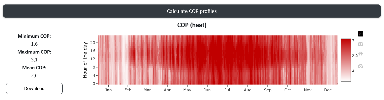
In nPro, the COP only depends on the source and sink temperatures, not on the load of the heat pump. The electricity demand in an hour is therefore , regardless of whether the heat pump operates at part load or at full output.
Carnot approach
With the Carnot approach, nPro calculates the COP from the sink and source temperatures in kelvin and the exergetic efficiency η:
You can choose an exergetic efficiency of 40 % (low efficiency), 50 % (medium efficiency) or 60 % (high efficiency), or a user-defined value. The COP is limited upwards to an adjustable maximum value and downwards to 1.1. If the sink temperature is not above the source temperature, the maximum value applies.
In cooling mode, the exergetic efficiency also refers to the Carnot COP of heating mode. The EER then results from the energy balance as COP − 1. The entered maximum value applies as the maximum EER, and the lower bound is an EER of 0.1.
COP from product data
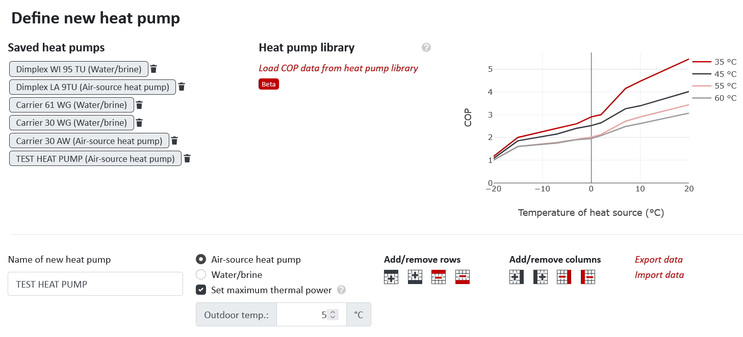
With product data, you enter the COP as a table: rows for the temperature of the heat source, columns for the temperature of the heat sink. nPro interpolates linearly between the table values in both dimensions. Outside the table range, the COP is held at the edge. The table should therefore cover the entire range of outdoor and flow temperatures and be filled in completely. A COP of 1.0 applies as the lower bound.
Using data sheet values
Data sheets of air-source heat pumps usually contain heating output, power input and COP for several outdoor and flow temperatures. For inverter heat pumps, these values are often given for maximum and minimum output, sometimes also for a nominal speed. When transferring them to nPro:
- Use the values at maximum output. Since the nominal electrical capacity in nPro is the maximum electricity consumption, the values at maximum output are the most consistent. At full load, output and electricity demand are then correct. At part load, the real efficiency is higher, so the seasonal performance factor in nPro tends to be conservative. Values at nominal speed, in contrast, are too optimistic at full load.
- Calculate the COP yourself if necessary. If the data sheet only states heating output and power input, the COP is the heating output divided by the power input.
- Keep the defrosting points. Values according to EN 14511 usually include defrosting losses around A2. This often shows as a higher power input at 2 °C than at −7 °C and 7 °C. Keep these points so that defrosting is taken into account via the interpolation.
- Complete grid. If individual values are missing in the data sheet, for example at high flow temperatures and very low outdoor temperatures, leave out the affected row or column. If the flow temperature of a sector then lies above the table range, the COP is held at the edge.
Heat pump models and library
Product data is saved as heat pump models, which can be used in all technologies that employ heat pumps. nPro contains five predefined models, two of which are air-source heat pumps (Dimplex LA 9TU, Carrier 30 AW). You create further models yourself: select the type (Air-source heat pump or Water/brine), enter the COP table or load the data from the heat pump library. Via Export data and Import data, models can be exchanged. If in doubt, check predefined values against the current manufacturer data sheet.
Output limit at high outdoor temperatures
Why the heating output reaches a plateau
According to the formula for the maximum heat output, it rises proportionally to the COP: a heat pump with an electrical capacity of 10 kW delivers at most 20 kW at a COP of 2, but already 60 kW at a COP of 6.
Real air-source heat pumps behave differently. With warmer outdoor air, the evaporating pressure and the refrigerant mass flow rise, and with them the heating output and the load on the compressor. To keep the compressor within its permissible operating range, the control limits the output, for example via the MOP function of the expansion valve on the suction side or via the speed if the high pressure rises too much. If that is not sufficient, the high-pressure switch trips and the heat pump cycles. The maximum heating output therefore remains roughly constant above a certain outdoor temperature, while the power input decreases.
This plateau occurs in principle with all air-source heat pumps. The outdoor temperature at which it takes effect, however, depends strongly on the device and may also lie outside the relevant temperature range.
Without a limit, the model overestimates the heat output in warm hours, i.e. mainly in the transitional season and in summer. The heat pump then covers too large a share of the demand, other generators are used too rarely, and the economic results are too favorable. This is most pronounced for demands that also occur at high outdoor temperatures, such as domestic hot water or process heat.
Representation in nPro: limit temperature per heat pump model
For an air-source heat pump model with product data, activate Specify max. heat output and enter a limit temperature of the outdoor air. From this, nPro determines the limiting COP, i.e. the COP at this temperature, and limits the heat output accordingly:
- Below the limit temperature, applies as before.
- Above the limit temperature, applies. The heat output remains constant, and the electricity demand decreases as the COP rises.
nPro calculates the limiting COP from the sector’s COP profile as the mean of the hours whose outdoor temperature is closest to the limit temperature. With a constant or sliding flow temperature, this equals the COP of the table at the limit temperature.
If the heat pump serves several sectors in the same hour, each sector takes up a share of the capacity, as if the heat pump switched between the sectors over time. The decisive value is the effective COP of the sector, i.e. the smaller of the COP of the hour and the limiting COP:
For sectors without a limit, the limiting COP is omitted and the COP or EER of the hour applies. The limit only applies to air-source heat pumps with product data. Sectors using the Carnot approach, a constant or an uploaded COP, as well as the cooling sector, are not limited.
Determining the limit temperature
The limit temperature is not simply the bend of the maximum curve in the data sheet. In real heat pumps, the power input at maximum output already decreases in the transition range, before the heating output reaches its plateau. nPro, in contrast, keeps the electrical capacity constant up to the limit temperature. The curve therefore rises faster than the data sheet curve and reaches the plateau output earlier (see Figure 4). The correct value is the outdoor temperature at which the nPro curve reaches the plateau output of the data sheet.
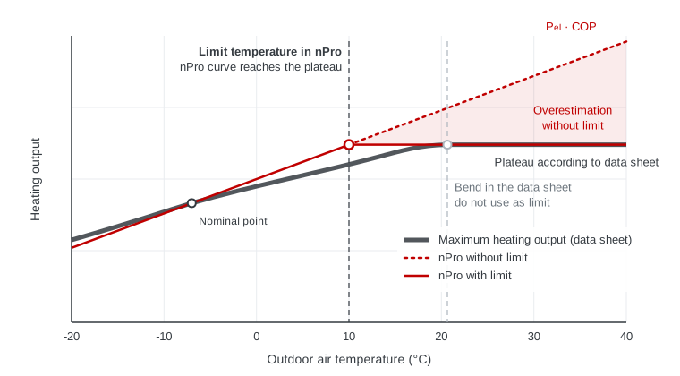
Proceed as follows:
- Determine the nominal electrical capacity from the chosen nominal point: .
- Read off the plateau output: the maximum heating output in the flat part of the curve, at the flow temperature of the sector.
- Calculate the limiting COP: .
- Determine the limit temperature: the outdoor temperature at which the COP table reaches this COP at the same flow temperature, interpolated linearly if necessary.
| Step | Value |
|---|---|
| Nominal point A−7/W35 (maximum output) | 45.8 kW, COP 2.79 |
| Nominal electrical capacity | 45.8 / 2.79 = 16.4 kW |
| Plateau output according to data sheet (from approx. 12 °C) | 61 kW |
| Limiting COP | 61 / 16.4 = 3.72 |
| COP table W35: 3.04 at 2 °C, 4.10 at 7 °C | Limit temperature ≈ 5 °C |
If the bend at 12 °C were entered in this example, the plateau in nPro would be at 16.4 kW · 4.63 = 76 kW, i.e. about 25 % above the data sheet.
In addition:
- The limit temperature and the nominal point belong together. With a different nominal point, the nominal electrical capacity changes and with it the matching limit temperature. In the example, it would be about 11 °C instead of 5 °C with A7/W35.
- Determine it separately for each flow temperature. At higher flow temperatures, the matching limit temperature is usually higher, and sometimes no limit is needed at all. If the heat pump serves several sectors with different flow temperatures, use a copy of the model with its own limit temperature for each sector.
- No limit is needed if the limiting COP is above the highest COP in the table. The nPro curve then does not reach the plateau within the table range.
Limit temperature and sizing
Since the limiting COP describes the ratio of plateau output to nominal electrical capacity, the limit scales with the capacity of the heat pump. It therefore also works when the capacity is optimized. The optimization assumes that a larger or smaller heat pump has the same characteristic curve shape as the device the data comes from. This applies to cascades of identical devices. Within a product series, however, the curves often differ considerably, and smaller models frequently reach the plateau at lower outdoor temperatures than larger ones.
If the sizing of the heat pump is of high importance, an iterative procedure is recommended:
- Restrict the optimization range to unit sizes with a similar characteristic curve.
- Run the optimization. With the recommended nominal point, the nominal thermal capacity equals the maximum output at A−7/W35 and can be compared directly with the unit sizes in the data sheet.
- Select the matching device or cascade and take over its COP table, nominal point and limit temperature.
- Repeat the calculation, if necessary with a fixed capacity. One or two runs are usually sufficient.
Operation and operational restrictions
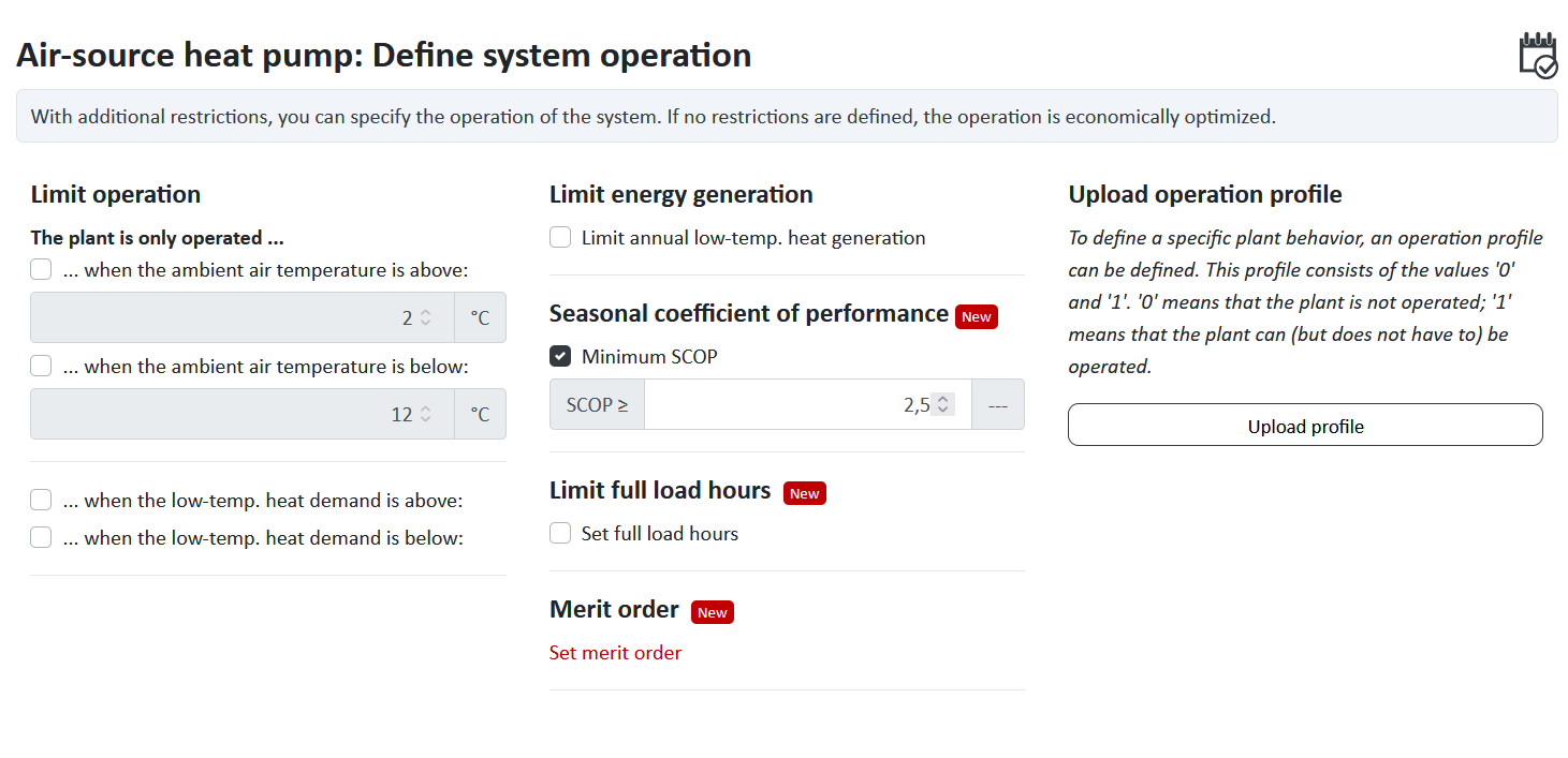
Without further specifications, the optimization determines the operation of the heat pump economically. In every hour, the heat pump can deliver any output between zero and its maximum output. Via the operational restrictions, you can restrict operation specifically. For air-source heat pumps, these options are particularly relevant:
- Outdoor air temperature above or below a value: represents the operating limit of the heat pump or a bivalence point.
- Minimum seasonal performance factor: ensures that the heat pump reaches a specified efficiency over the year, for example as a requirement from funding conditions.
- Full-load hours: limit or enforce a certain utilization.
- Merit order: defines the ranking in which the heat pump and other generators are used. Examples of bivalent alternative, parallel and partly parallel operation can be found on the merit order page.
Active restrictions are shown in the input form of the air-source heat pump.
Results
In the sizing of the plants, nPro shows for the air-source heat pump:
- Nominal thermal capacity and electrical capacity, e.g. 272 kWth at COP = 4 (68 kWel). The nominal thermal capacity is the optimized electrical capacity times the nominal COP.
- Maximum heat output per temperature level, e.g. = 156 kWth at COP = 2.3. This is the highest heat output the heat pump delivers at this temperature level over the year, together with the COP of that hour. If several hours reach this output, the lowest COP is shown. If it is clearly below the nominal thermal capacity, the nominal COP was set at a more favorable operating point than the hours with the highest demand.

The seasonal performance factor of the air-source heat pump is shown in the results of the operational simulation.
Limitations of the model
nPro deliberately models the air-source heat pump in a simplified way for conceptual design:
- Constant electrical capacity. The maximum electricity consumption does not change with the outdoor or flow temperature. In reality it varies, so the maximum output is exact at the nominal point and deviates at other temperatures. The limit temperature compensates for this in the warm range.
- One COP per operating point. The COP does not depend on compressor speed or load. Which speed is represented depends on the values entered.
- Defrosting. Defrosting losses are not calculated separately. They are included insofar as the COP values account for them.
- Operating behavior. Minimum output, cycling and running times are not represented.
The heat source is the outdoor temperature from the weather data of the location.