Sizing of geothermal borehole fields: Calculation and validation

System design: Geothermal boreholes with heat pumps

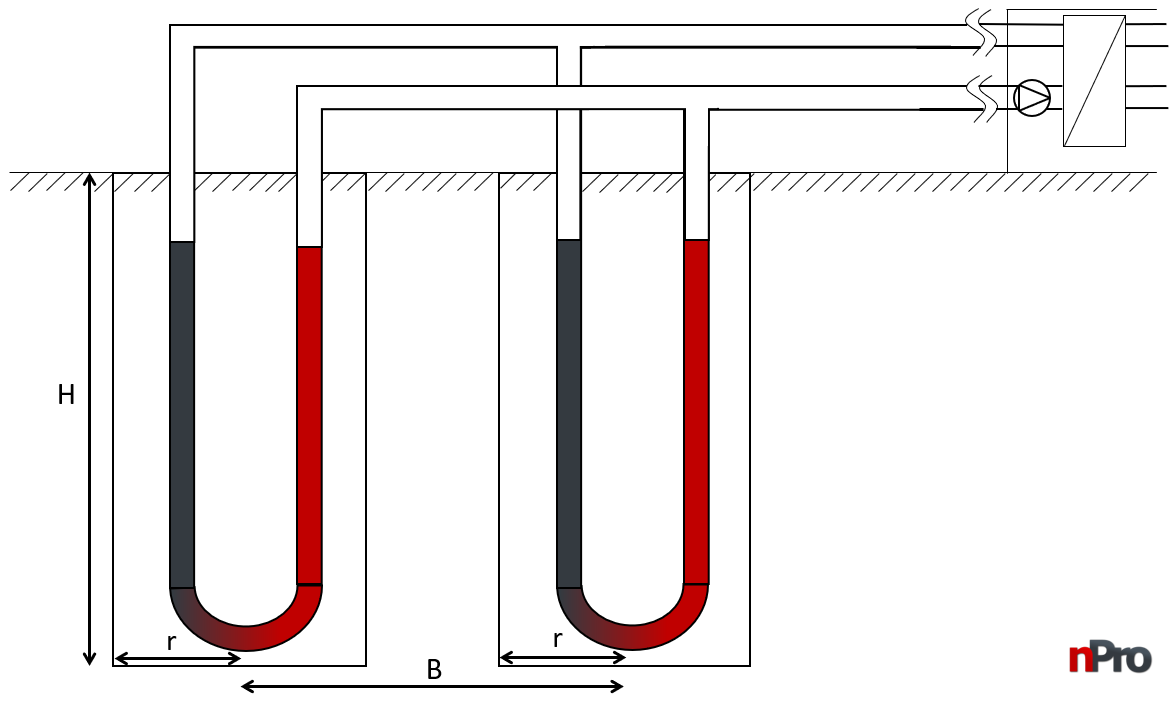
To exploit the underground thermal potential, various technologies such as heat pumps or heat exchangers can be used. They supply either individual buildings or entire districts via a heat network. In Figure 1, the connection between the heat pump or heat exchanger and the geothermal borehole extracting heat from the ground is illustrated. The dimensions of the borehole are crucial for the calculation of heat yield. The borehole length (H) defines the depth to which the geothermal probe reaches into the ground. The borehole spacing (B) indicates the horizontal distance between two boreholes and it influences the efficiency of heat extraction. The borehole radius (r) is significant as it affects the contact area between the soil and the probe. These probe parameters are central to designing an efficient geothermal borehole system as they significantly influence the extraction of geothermal energy.

Methods for geothermal borehole calculation

The calculation basis used in nPro for geothermal borehole fields is based on the work of Prof. Koenigsdorff from the Hochschule Biberach (Germany). It employs models based on the work of the Swedish scientists Eskilson and Hellström, taking into account three load conditions: base load, periodic load, and peak load. The base load represents the average, continuous heat demand throughout the year, while the periodic load reflects monthly fluctuations in heat demand due to seasonal temperature differences. The peak load describes the maximum heat demand in extremely cold periods (coldest hours of the year). Crucial in the calculation is the calculation of fluid temperatures in the probes and their influence on the soil. These calculations are essential to avoid overloading of the geothermal probe field or undesired temperature changes in the ground. Prof. Koenigsdorff has developed the software GEO-HAND^light and validated the results of his calculation methodology with the well-known software Energy Earth Designer (EED) and the German guideline VDI 4640. To determine the thermal resistance of the base load, the g-function introduced by Eskilson is used. This is a thermal step response to heat transfer and considers the interaction between individual boreholes. Different to Koenigsdorff’s calculation, nPro uses an open-source simulation core for calculating the g-function, which was developed as part of the doctoral thesis by Massimo Cimmino (today professor at École polytechnique de Montréal in Canada). Detailed information on the calculation basis can be found in the book “Oberflächennahe Geothermie für Gebäude” by Prof. Koenigsdorff, as well as in the user manual for the GEO-HAND^light program (version 5.0). The source code of Prof. Cimmino’s open-source computational core is available in the public code repository pygfunction on Github.

How to design a geothermal borehole field with nPro?

The geothermal module in nPro provides 4 essential calculation functions:

• The calculation of the number of boreholes depending on the specified borehole length, temperature at the heat pump outlet, and borehole spacing.

• The calculation of the borehole length depending on the borehole arrangement, borehole spacing, and the temperature at the heat pump outlet.

• The calculation of the temperature at the heat pump outlet depending on a given borehole length, the borehole spacing and the borehole arrangement.

• The calculation of the temperature profiles at the heat pump outlet depending on the given borehole length, the borehole spacing and the borehole arrangement.

For the borehole calculation, nPro uses the extraction profiles calculated in the operation simulation, the air temperature profile based on the selected location and an assumed peak load duration of 4 hours. A rectangular arrangement of the boreholes is assumed for the calculation.

Validation with EED (Energy Earth Designer)

In the following, the sizing of geothermal probes in nPro will be compared exemplarily with the calculation results from EED (Energy Earth Designer) using two calculation examples. EED is a standard software for geothermal design. For the calculation of the g-function, nPro standardly uses the boundary condition of a uniform borehole wall temperature (UBWT).

The deviations between the calculation results of nPro and EED are small. In the first load case, the probe length deviation is 2 meters (138 meters in nPro instead of 140 meters in EED), and in the second load case, it is 8 meters (148 meters in nPro instead of 140 meters in EED). The relative deviations are 1.4 % in the first load case and 5.7 % in the second load case. These deviations result, among other factors, from the different calculation methods for the g-function. In nPro, the g-function is geometrically calculated using the pygfunction calculation core developed by Massimo Cimmino. Overall, the discrepancies between both software tools are acceptable (approximately 5 - 10 %), especially when considering that the uncertainty of input parameters in the early planning phase of a geothermal system is significantly greater.

Validation with GEO-HAND^light

In addition to the validation with EED, the calculation methodology of nPro was compared to GEO-HAND^light (Version 5.0) by Prof. Koenigsdorff. In this validation, the boundary condition of a uniform heat transfer rate (UHTR) was used to calculate the g-function. In the current version of nPro, on the other hand, the boundary condition of a uniform borehole wall temperature (UBWT) is used by default. This results in slight differences in the calculation of the g-function.

Validation of the borehole length

The following section compares the sizing of geothermal boreholes in nPro with the calculation results from the GEO-HAND^light tool (version 5.0) by Prof. Koenigsdorff.

Definition of validation scenarios

Validation of the probe length calculation

For various rectangular borehole arrangements, the borehole lengths calculated with nPro and GEO-HAND^light are compared. The deviation results from different methods used to determine the g-function (nPro calculates the g-function geometrically using the simulation core of Massimo Cimmino, while GEO-HAND^light uses heuristic calculation approaches). Overall, the differences between both tools are insignificant (below 3 % in most cases).

Validation of the calculation of the temperature at the heat pump outlet

To calculate the number of probes, nPro uses the heat pump outlet temperature as a design criterion. Consequently, the heat pump outlet temperature in nPro is compared to that of the GEO-HAND^light tool. A validation of the number of probes is not possible since it cannot be directly determined using the GEO-HAND^light tool.

Validation with Scientific Study

In addition to the validations with EED and GEO-HAND^light, the calculation results from nPro were compared with those of a scientific study that evaluated 12 software tools for geothermal borehole field sizing, including an intermodel comparison (Ahmadfard et al.: A review of vertical ground heat exchanger sizing tools including an intermodel comparison, Renewable and Sustainable Energy Reviews, 2019) [8]. This validation used a temperature difference condition of 3 K between the inlet and outlet of the borehole to calculate the borehole length. The following compares the dimensioning of geothermal boreholes in nPro with the calculation results from the study.

Methodology for determining the probe (borehole) length

To determine the probe length, it is assumed that all probes in the geothermal field are of equal length and hydraulically connected in parallel. The calculation utilizes an iterative approach since the values of the borehole resistance of the base load and the temperature response in the formula to calculate the probe length again depend on the probe length. The iteration continues until the difference between the newly calculated length and the previously calculated length is less than 1 meter. The results of this calculation methodology have been validated with the German guideline VDI 4640 Part 2 in a work by Prof. Koenigsdorff. nPro employs the same calculation approach.

• Calculation basis: $\begin{gathered} H= \frac{Q_{Net base load} \cdot (R_{Base load} + R_{B}) + Q_{per} \cdot (R_{per} + R_{B}) + Q_{peak} \cdot (R_{peak} + R_{B})}{\Delta T_{Reaction} \cdot N_{Number of probes}} \end{gathered}$

As an add-on to the Koenigsdorff calculation method, nPro also offers the option of designing the probes under dominant cooling load. If the cooling demand is decisive for the design due to high periodic loads and peak loads (or a low maximum probe outlet temperature) compared to the heat demand, the necessary probe length is designed using the cooling load. In this way, excessively high temperatures at the probe outlet can be avoided.

Calculation of the heat pump outlet temperature

The heat pump outlet temperature corresponds to the temperature of the heat transfer fluid at the probe inlet. Together with the temperature difference, it indicates the state of the fluid before and after passing through the probe. The higher the temperature at the probe outlet, the higher the efficiency of the heat pump. The minimum heat pump outlet temperature, which is set in a steady state and is only reached after several decades, is decisive for the design. This steady-state temperature can be determined by the calculation approach.

• Calculation basis: $\begin{gathered} T_{HP,out}= T_{Undisturbed soil} + \Delta T_{Base load} + \Delta T_{per} + \Delta T_{peak} - 0.5 \Delta T_{Fluid} \end{gathered}$

Validated value ranges and determination of input values

This section explains which values can be used for the input parameters for the borehole field calculation and from where suitable values can be obtained.

Determination of borehole resistance and thermal conductivity

Backfill materials for ground probes can be categorized into conventional and thermally enhanced materials. On average, conventional materials have an increased mean resistance of about 0.1 (mK)/W compared to thermally enhanced materials, which have approximately 0.08 (mK)/W. Additionally, there is an increase in thermal resistance with increasing borehole radius (refer to the overview on geoenergie-konzept.de).

Sources