Energy center: sizing plants and simulating operation

From the demand to its optimal coverage

Once the energy demands have been calculated – for an entire district or for a single building – the energy center module answers the question of how to cover them optimally. If the demands are already available, for example as specified by the client or as the result of another software, they can just as easily be reused (see the energy center project). How nPro determines the demands itself is described under load profiles and demand simulation.

The path there leads through five steps, which this page describes one after the other:

1. Assembling the generator portfolio: which technologies are eligible in the first place?
2. Configuring the plants: how are they adapted to the actual conditions?
3. Defining the boundary conditions: which costs, subsidies and objectives apply?
4. Sizing the plants: which capacities are optimal?
5. Simulating and evaluating the operation: how is the system operated over the year?

Extensive generator portfolio

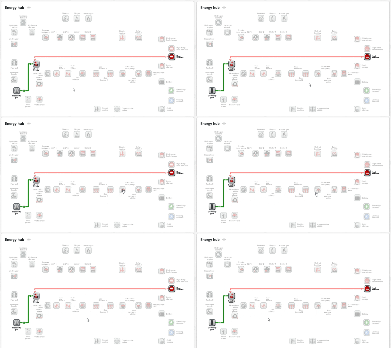
In the first step, it is defined which generators are to be considered at all. In nPro, this is done intuitively: a click on the graphic of a generator selects or deselects it (see Figure 1).

How extensive the selection is can be seen from the example of the heating demand. The following technology groups are available to cover it (see Figure 2):

• Solar generation: solar thermal and PVT collectors, which provide heat and electricity at the same time.
• Ambient heat and geothermal energy: freely definable heat sources such as waste heat, river or wastewater heat as well as geothermal energy via borehole heat exchangers. If the temperature level of the source is not sufficient, a downstream heat pump raises the heat to the required level (“boosting”).
• Heat pumps: in various designs, depending on the source used – from the air-source heat pump to a heat pump connected to a previously defined heat source.
• Waste heat from sector coupling: the waste heat of an electrolyzer or a fuel cell, which arises as a by-product of hydrogen use anyway.
• Fuel-based generators and power-to-heat: boilers, CHP units and electric heating elements, typically for medium and peak load as well as to safeguard the supply.
• Grid-bound purchase: district heating as externally purchased heat.
• Thermal storage: to decouple generation and demand in time, whereby the storage losses are also calculated.

The heating demand can be split into a low-temperature and a high-temperature demand; in a district project, this happens automatically via a threshold temperature if desired. This separation is always useful when different technologies are intended for the two levels: in a new-build district with panel heating, for example, a heat pump covers the space heating at a low temperature level particularly efficiently, while the domestic hot water requires a considerably higher level and is provided by a separate generator – such as an electric heating element or a CHP unit. How nPro handles temperature levels is described under heating curves.

The options for covering cooling, electricity and hydrogen demand are just as extensive. Sector coupling is consistently taken into account: an absorption chiller generates cooling from heat that comes, for example, from a CHP unit or the solar thermal system; an electrolyzer converts surplus PV electricity into hydrogen and provides its waste heat to the heating network; a fuel cell in turn generates electricity and heat from hydrogen. Storage units for heat, cooling, electricity and hydrogen shift generation in time to where it is most favorable. Examples of such coupled systems can be found under hydrogen in districts and in the hydrogen case study.

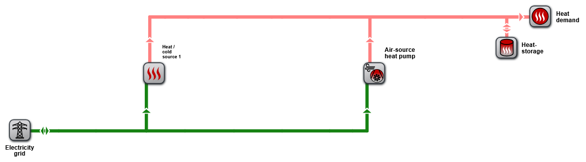
In the following, the supply of a residential development with waste heat from a data center as well as an air-source heat pump in combination with a thermal storage unit serves as a running example. For this, a heat source, an air-source heat pump and a thermal storage unit are selected in nPro, as Figure 3 shows.

Plant configuration in detail

Once the generator portfolio has been determined, it is advisable to configure the individual generators in detail. In nPro, all parameters are already populated with sensible default values, but can easily be adjusted; numerous tooltips provide additional explanations. Figure 4 shows, as an example, the input form for the heat source parameters before and after configuration.

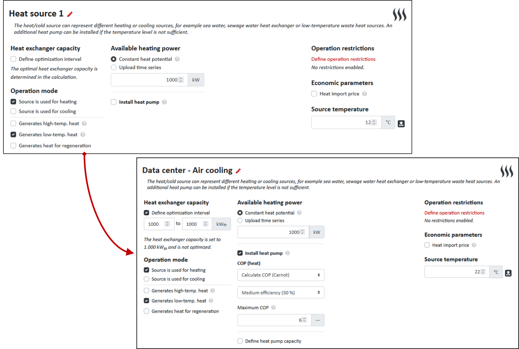
In this way, the generators can be brought step by step closer to the actual conditions. In the example, the waste heat from the air cooling of a data center is to be used, which is why the designation of the generator is changed first. The potentials have been estimated by the operator of the data center; they are entered directly into the form. Instead of a constant potential, a time series could also be uploaded – useful, for example, for weather-dependent sources such as a river. The same approach can be taken for the source temperature.

Since the source temperature is not sufficient to cover the heating demand, a heat pump is used for boosting. In the example, its COP is determined via the Carnot efficiency; alternatively, manufacturer data could be entered. The thermal capacity at the condenser initially remains unknown and is determined later by the plant sizing, while the capacity at the evaporator is constrained by the heat source potential and the heat exchanger capacity.

In addition to these generator-specific settings, nPro also allows operational restrictions to be specified (see Figure 5), which can considerably influence the operation.

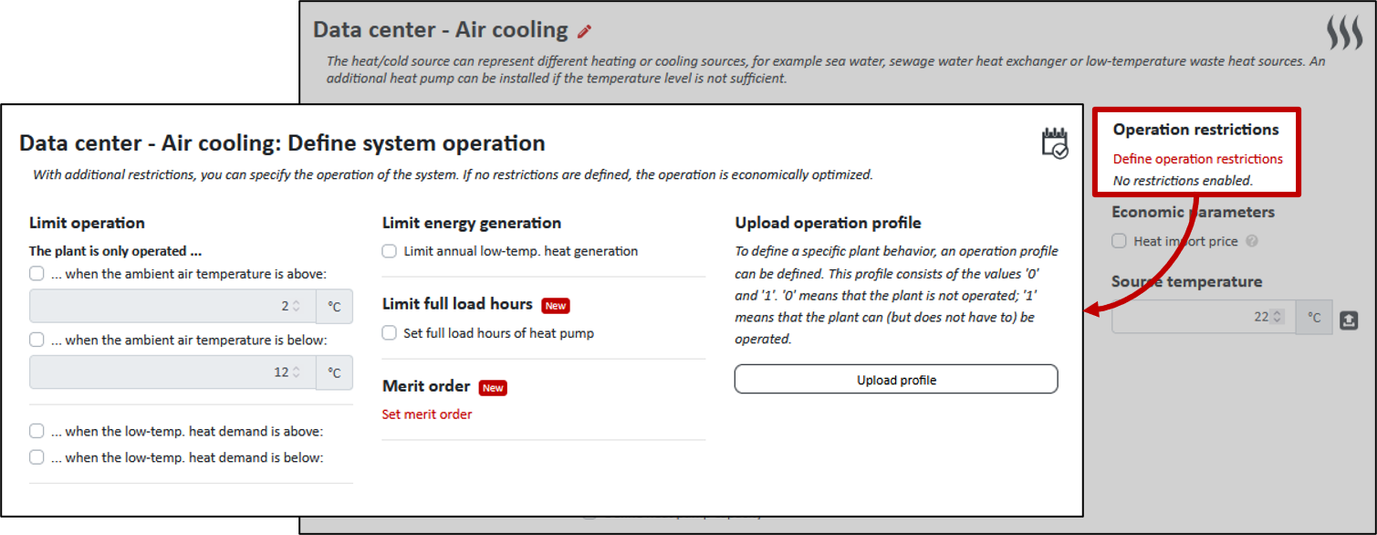
For example, an operating profile can be uploaded in order to represent planned outages, or conditions can be defined under which the generator may be operated on its own.

Economic and environmental boundary conditions

The economic and environmental settings are just as extensive as the technical ones. Figure 6 shows the corresponding buttons. The following can be configured:

• Energy purchases: how expensive is the purchase? What remuneration is there for feed-in? Are there purchase or feed-in restrictions?
• Technology costs: investment and maintenance costs, subsidies, service life as well as the question of whether a plant is part of the existing stock.
• General economic settings: parameters of the net present value calculation, annual price changes, the CO₂ price and the operating cost subsidy according to BEW.
• General environmental settings: emission and primary energy factors, savings targets for the optimization as well as coverage shares for generator groups.
• General optimization settings: among other things the objective to be minimized and the specification of a merit order; the background to this is described by the optimization model.

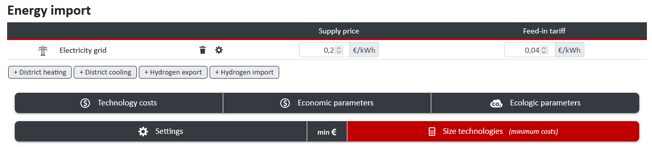
These settings determine very concretely which solution the plant sizing and the subsequent operational simulation deliver. Four of them are singled out in the following: the specific investment costs, the coverage share of generator groups, the merit order and the choice of the optimization objective.

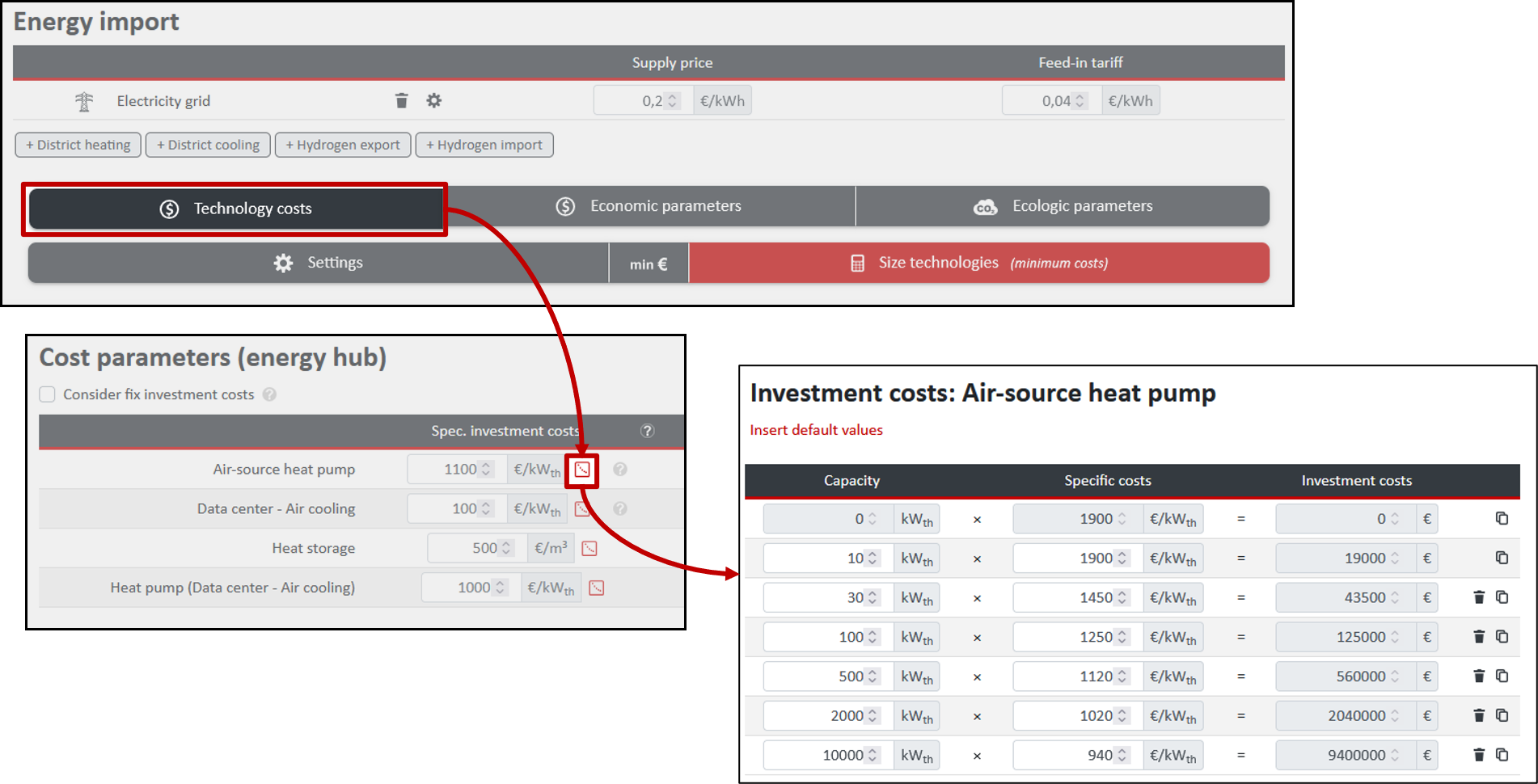
The specific investment costs can be specified in nPro linearly or non-linearly. Linear means that the investment costs increase proportionally with the plant size. In reality, however, economies of scale often occur, through which the specific costs decrease as the plant size grows. For a non-linear cost function, a click on the small button next to the field for the linear costs is sufficient; behind it lie the modifiable default values of the cost function (see Figure 7).

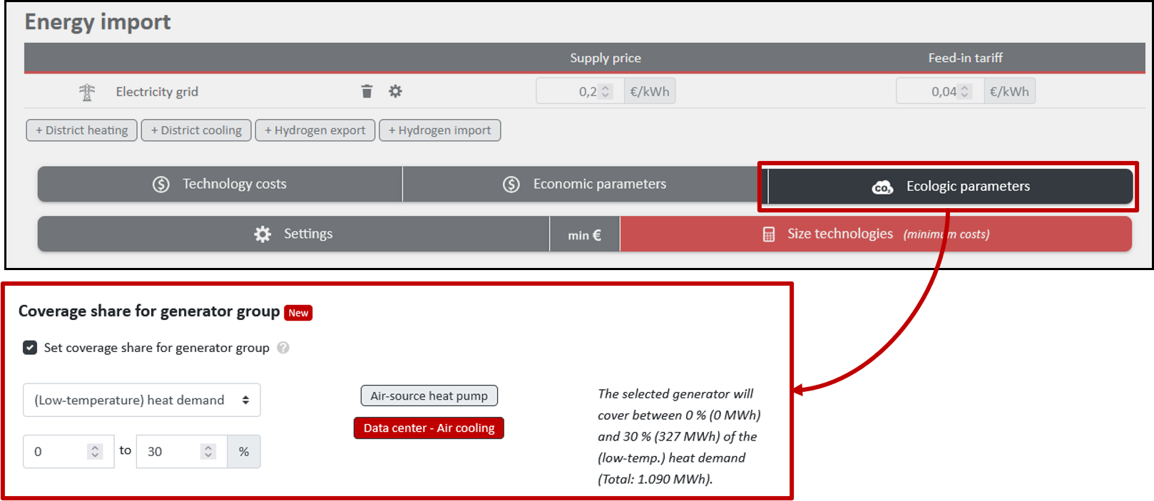
Via the coverage share of generator groups, several generators can be combined into a group and this group assigned a share of the total generation (see Figure 8). The specification acts as a constraint in the optimization: the group must comply with the required share, even if a different allocation would be more cost-effective. Typical use cases are demonstrating a minimum share of renewable heat, as required by legal regulations or funding programs such as the BEW, or conversely limiting a share – for example when only a certain amount of fuel per year is available for a biomass CHP unit. The setting can be reached via the environmental parameters.

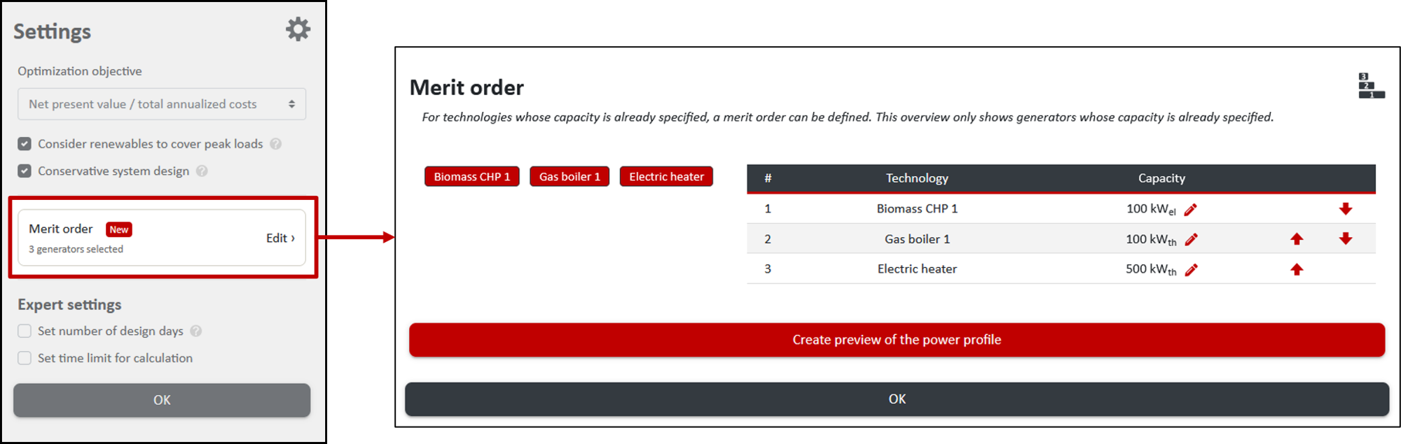
The merit order defines the sequence in which the generators are called upon to cover the load: only once the higher-priority generator has exhausted its capacity does the next one switch on. Instead of a purely cost-optimal operating strategy, this results in rule-based and therefore easily traceable operation, corresponding to the usual division into base, medium and peak load. Figure 9 shows this for a system consisting of a biomass CHP unit, a natural gas boiler and an electric heating element: the CHP unit covers the base load, the boiler steps in at higher loads, and the electric heating element safeguards the peaks. The order can be set via the operational restrictions of the individual generators or via the general settings menu – however, only for heat generators whose capacity is limited.

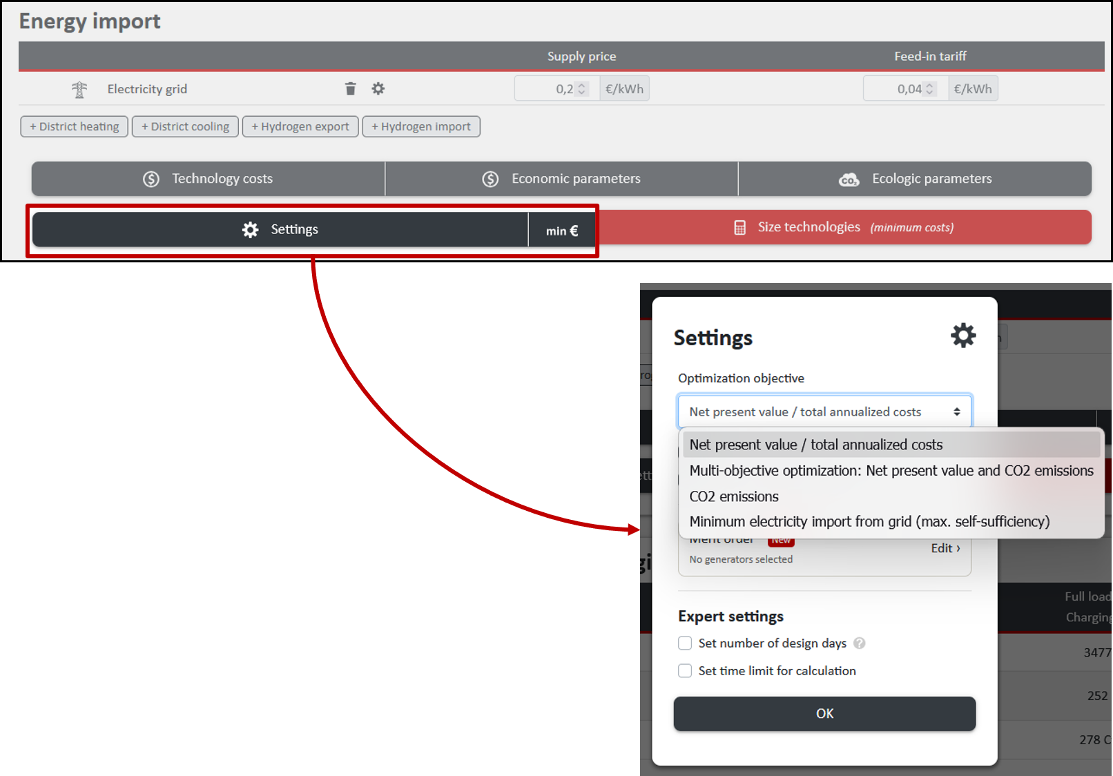
The optimization objective for the plant sizing and the operational simulation is also chosen via the general settings (see Figure 10). The following options are available:

• Net present value or annualized total costs
• Multi-objective optimization: net present value and CO₂ emissions
• CO₂ emissions
• Minimum electricity purchase from the grid (maximum self-sufficiency)

Sizing the plants

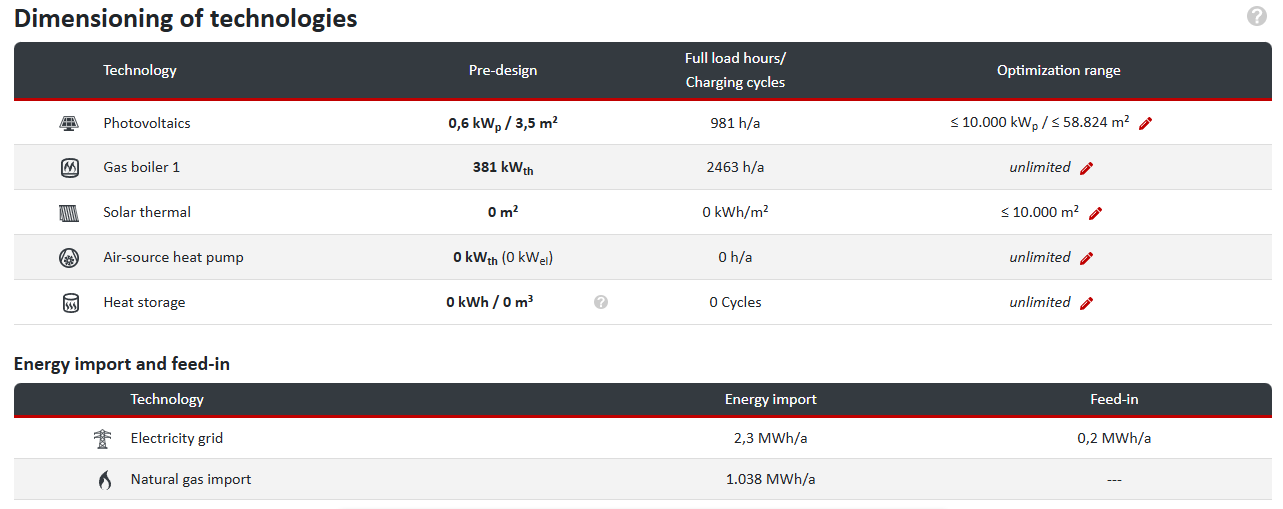
For the optimal plant sizing, a click on the corresponding button is sufficient (see Figure 6). Depending on the technical parameters and the costs entered for the various purchase sources, the optimization model determines the optimal capacities of the available technologies for covering the energy demands. An example result for a system consisting of a natural gas boiler, an air-source heat pump, a solar thermal system, photovoltaics and a thermal storage unit is shown in Figure 11; in this example, the solar thermal system is required to have a collector area of at least 250 m².

It should be noted that a very extensive use of restrictions can lead to a situation in which no valid solution exists any more. In this case, nPro points out the restrictions responsible.

If the requirements change over the course of the project – for example regarding the share of renewable energies – or the framework conditions change – for example the areas available for photovoltaics or the space capacities for the thermal storage unit – the individual plants can be readjusted and resized quickly.

Operational simulation

Once the plant sizing is satisfactory, Simulate system operation starts the simulation of the energy system with fixed technologies and generates an energy flow diagram.

The thickness of the energy flow lines is proportional to the amount of energy transferred, which is additionally displayed when hovering over them with the mouse pointer (see Figure 12).

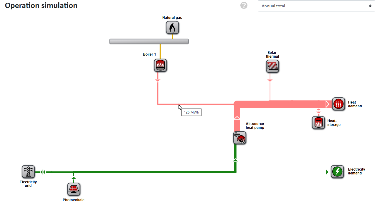
The period represented by the energy flow diagram can be freely selected: the annual total, the winter or summer half-year, the four seasons as well as individual calendar months. In the present example, the heat comes more from the solar thermal system in summer and less from the natural gas boiler – when the summer half-year is selected, the corresponding energy flow lines therefore become thicker and thinner respectively.

Various evaluations are available below the diagram:

• Electricity balance
• Heat balance
• Hydrogen balance
• Electricity grid: purchase and feed-in
• Renewable energies
• Energy demands

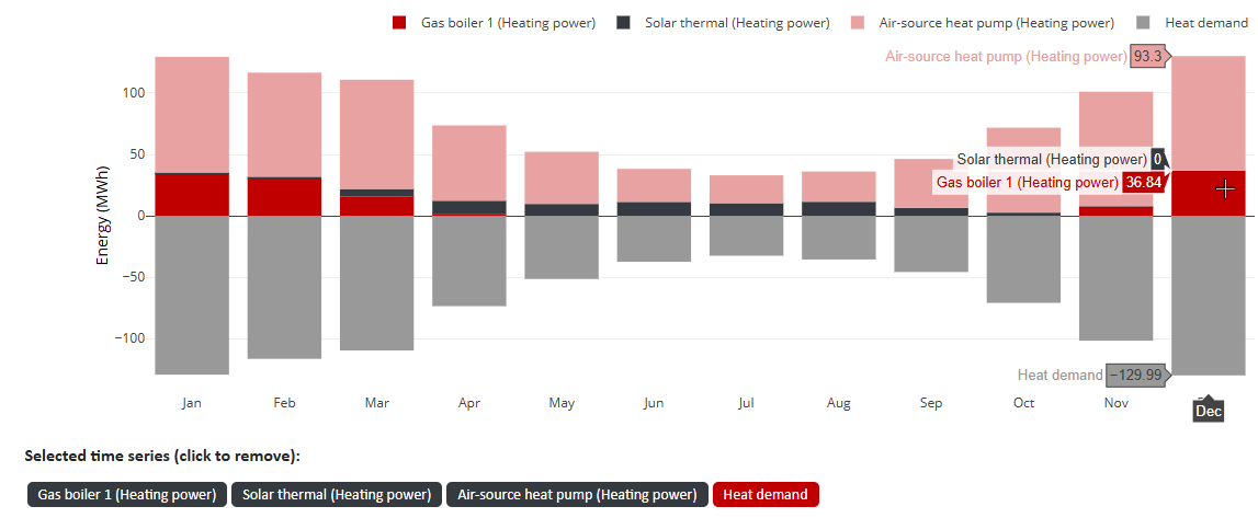
Here, too, the profiles can be displayed as a monthly or annual profile, as an annual load duration curve as well as a heat map (see Figure 13). In the monthly profile it is clearly apparent that the natural gas boiler is operated mainly in winter and the solar thermal system mainly in summer, while the air-source heat pump works all year round.

The heat map (see Figure 14) shows that the air-source heat pump supports the natural gas boiler in winter, whereas in summer it primarily runs during the day when the photovoltaic system produces electricity. At night, its operation is strongly reduced.

The operating strategy simulated by nPro therefore optimizes the use of the air-source heat pump in this example: it preferentially runs at times of high and therefore inexpensive PV electricity generation. As a result, low-cost electricity is used and, thanks to the higher outside air temperatures during the day, a higher COP is achieved at the same time (see also system COP).

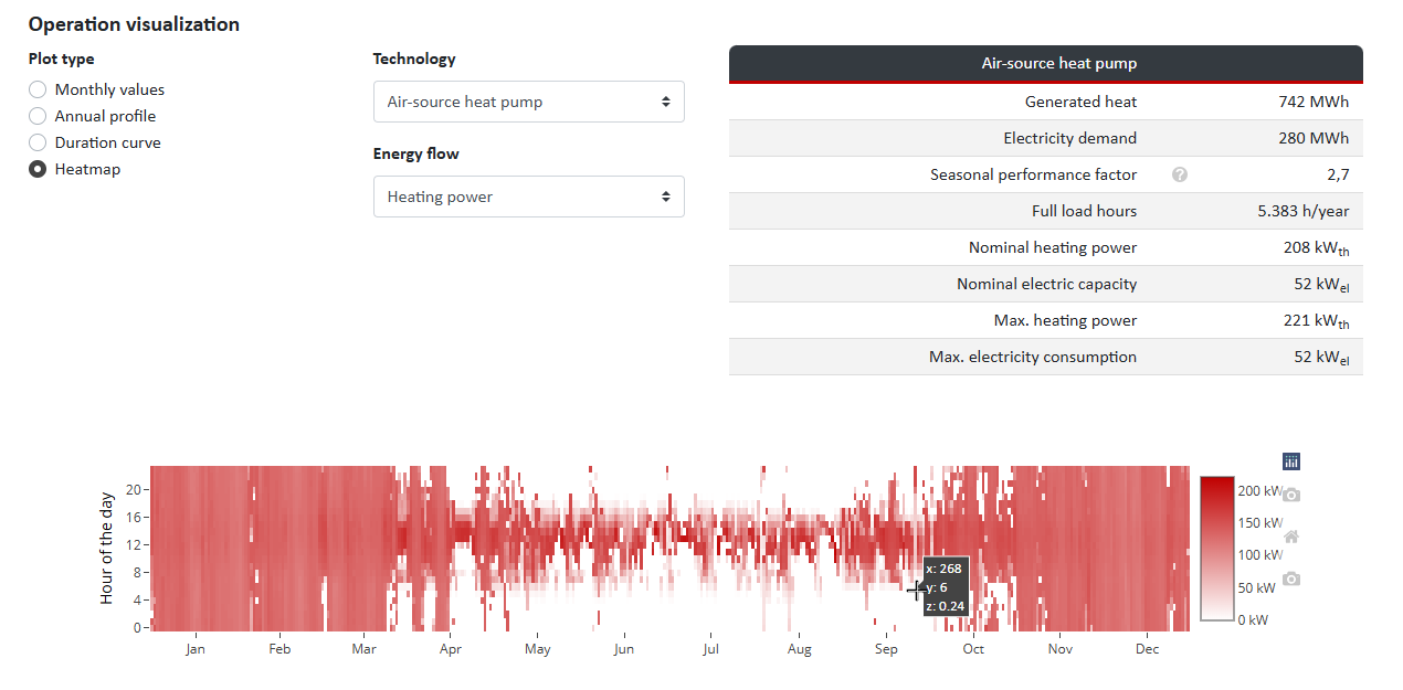
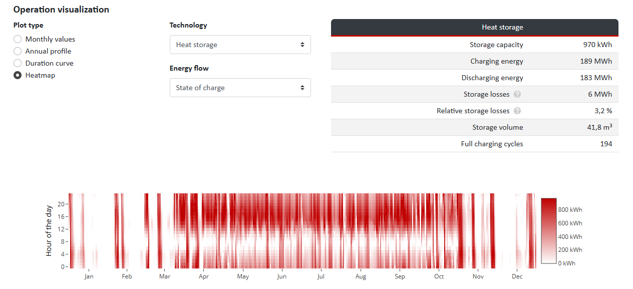
By selecting further technologies and visualizations, the interplay of the energy sources and their dependence on the time of day and season can be traced even more precisely (see Figure 15).

Overview of results

The overview of results summarizes the most important key figures and presents them graphically. In particular, the following are taken into account:

• Energy purchase:
  • Electricity purchase from the grid
  • Renewable electricity generation
  • Natural gas
  • Heat from the solar thermal system
• Energy feed-in
• Electricity generation and electricity purchase:
  • Renewable electricity generation (various sources)
  • Electricity purchase from the grid
  • Self-sufficiency rate
  • Self-consumption rate
• Heat generation and heat purchase:
  • Various technologies
  • Solar thermal coverage ratio (see Figure 16)
• Emissions:
  • Electricity purchase
  • Electricity feed-in
  • Natural gas
• Primary energy:
  • Electricity purchase
  • Electricity feed-in
  • Natural gas
• Energy demands:
  • Electricity demand
  • Heating demand

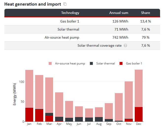
The complete economic evaluation of the system – net present value, payback period, levelized cost of heat and the breakdown of all cost items – then takes place in the results section; the methodological background is described by the economic feasibility calculation.