In this case study, a district with heating and cooling demands is supplied via a 5GDHC network. The entire planning process can be carried out in the nPro tool: from demand calculation to pipe dimensioning to the design of heat and cooling generators in the energy center.

District

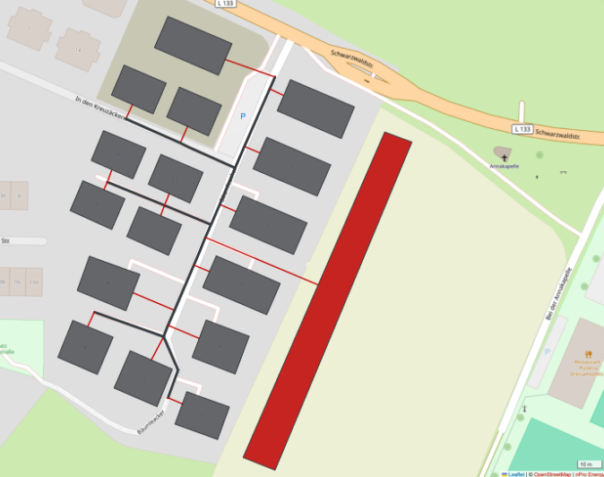
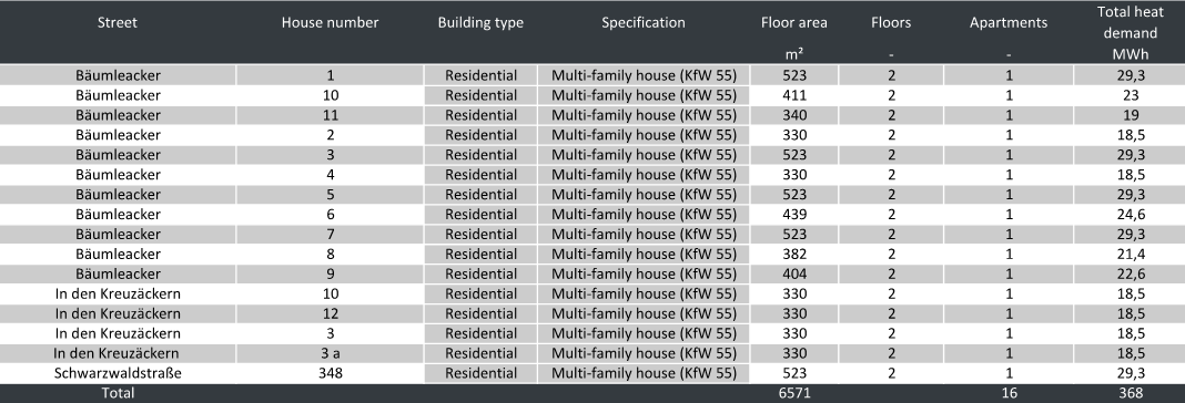
A district energy system is planned for a district with 16 buildings in Freiburg (Germany). Weather data for the Freiburg location is used for the simulation.

Figure 1: District with the 16 buildings to be supplied. Geothermal boreholes on a free area east of the district are planned as the heat source.

Step 1: Determine heating and cooling demands

Building standard:

KfW 55

Heat source/energy center:

Geothermal boreholes

Space heating and domestic hot water demand:
- Coverage using brine-water heat pumps from the 5GDHC network
Peak load:
- Coverage using electric heaters in heat pumps
Heat pumps:
- Calculation using COP characteristic curves stored in nPro for various heat pump manufacturers
Cooling demand:
- Coverage using heat exchangers (passive) → Discharge of waste heat into the heating network
Electricity:
- Includes: operating electricity of decentralized heat pumps
- Not included in this case study: user electricity (e.g., lighting) and e-mobility

Annual profiles with hourly resolution are crucial for district design, as time- and season-dependent renewable sources (here photovoltaics) are used.

Table 1: Building overview of the district to be supplied as an Excel export from nPro

Step 2: Pipe dimensioning

For design with decentralized pumps, the following assumptions apply:

Maximum delivery head: 80,000 Pa
Pressure losses due to pipe fittings: 25%
Heating network: directed heating network
Waste heat injection: with a temperature spread of 5 K

The entire heating network can be dimensioned automatically using nPro. In this case study, the assumptions shown in Figure 2 are used for the network calculation.

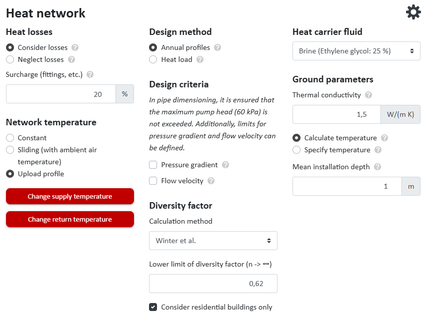
Assumptions for the heating network calculation

Figure 2: Settings for the heat network calculation in nPro

Figure 3 illustrates the dimensioning of the heating network after adding all buildings to the district. Once the pipe parameters are entered, nPro calculates the optimal pipe dimensioning for each network section for the passive 5GDHC network.

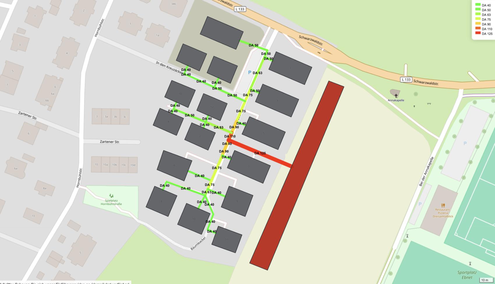
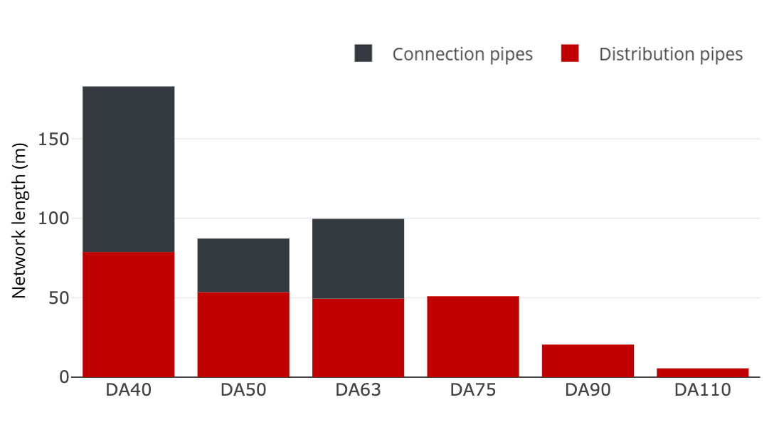
Map: Pipe dimensioning of the heating network

Figure 3: Pipe dimensioning of the 5GDHC network in nPro

The distribution of various pipe diameters can be displayed in nPro not only cartographically but also diagrammatically, see Figure 4.

Figure 4: Distribution of pipe diameters for the 5GDHC network

In the nPro tool, pipe diameters for 5GDHC networks can be automatically calculated.

After dimensioning and simulation, the results can be displayed in nPro: Figure 5 shows the heating loads of the buildings as well as the maximum thermal loads in individual pipe sections. Due to decentralized heat pumps, the loads in the building connection pipes are lower than the heating loads of the buildings.

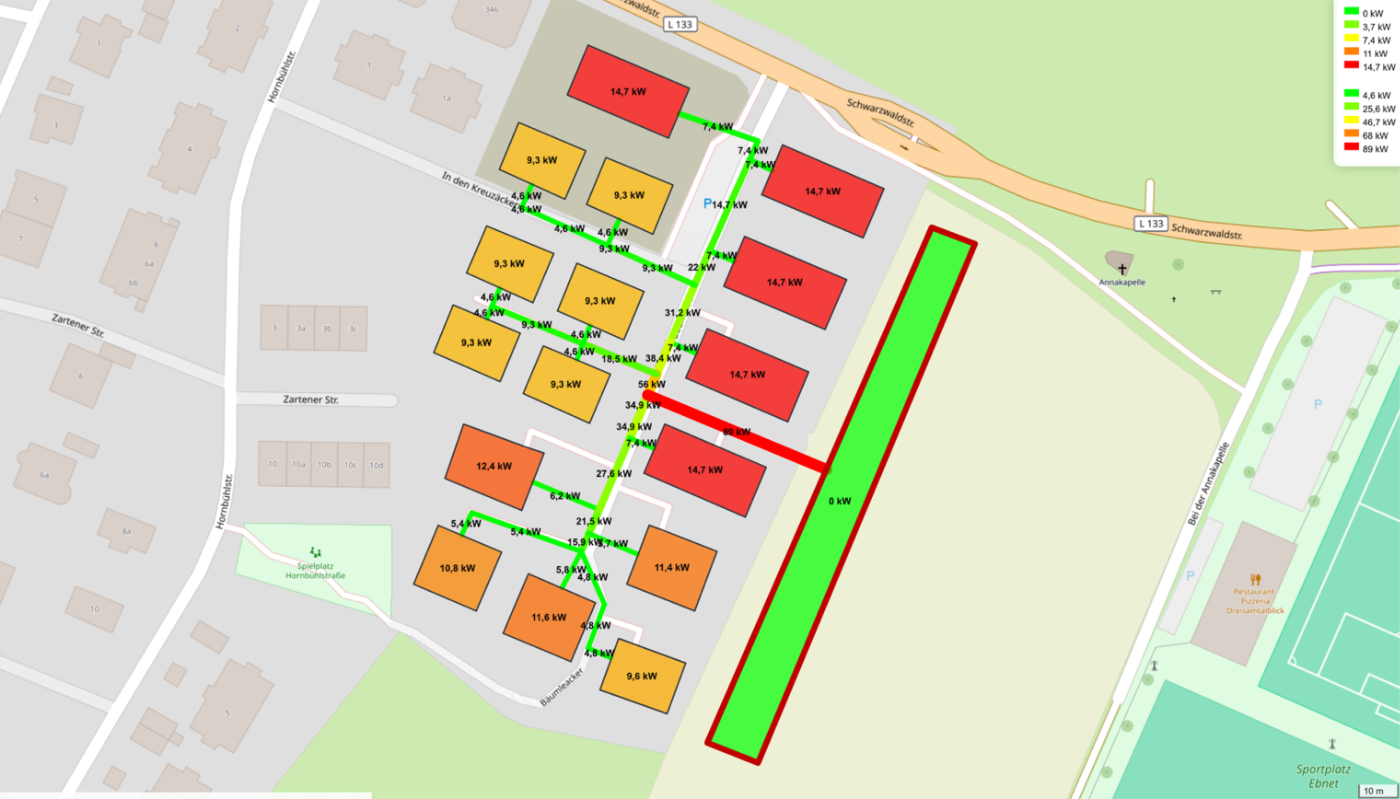
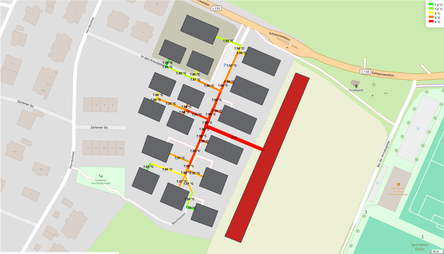
Map: Total heating demand (buildings), maximum transferable power (pipe sections)

Figure 5: Heating loads of the buildings and the maximum thermal loads in the individual pipe sections

Figure 6 shows the supply temperatures in the 5GDHC network.

Figure 6: Result of the network temperature calculation: supply temperatures in the 5GDHC network

Step 3: Load at the energy center

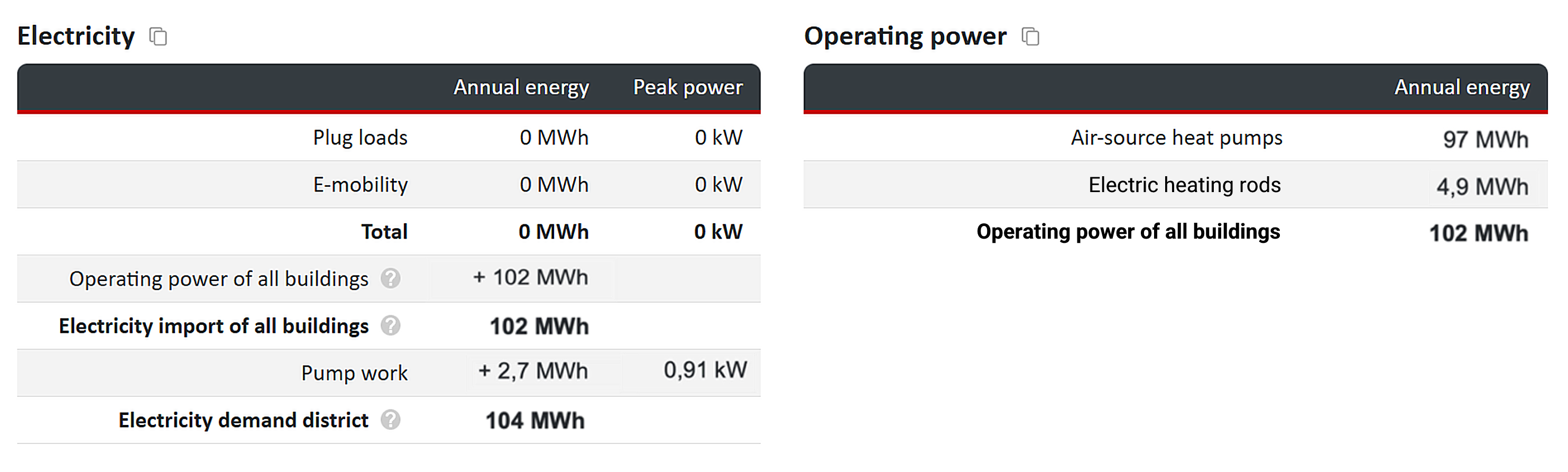
nPro calculates the heat and cooling demand of the district and at the energy center. Table 2 shows the heat (or cooling) demands of the 5GDHC system as well as the electricity demands of the operating power of the decentral heat pumps. The heat imported by the buildings from the 5GDHC network is (here at 91 kW) lower than the actual total heating demands (here at 185 kW), as the heat pump evaporator demand is lower than the heat pump condenser power.

nPro Tool: Annual energy demands for heating and cooling

Table 2: Heating and cooling balance for 5GDHC network

nPro Tool: Annual energy demand for electricity

Table 3: Electricity balance for the 5GDHC system (due to the operating power demand of the heat pumps)

Balancing effects of heating and cooling demand

If heating and cooling demands occur simultaneously, waste heat from the cooling provision can be directly utilized at the heat pump evaporator. Thus, simultaneous heat and cooling demands can partially cancel each other out. This balancing effect in the building or the 5GDHC network is automatically considered in nPro during the hourly calculation. Figure 7 shows the heating and cooling demand profiles at the energy center.

Heat and cooling loads at the energy center

Figure 7: Heating and cooling loads at the energy center

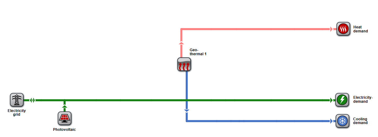
Step 4: Design of the geothermal borehole field (energy center)

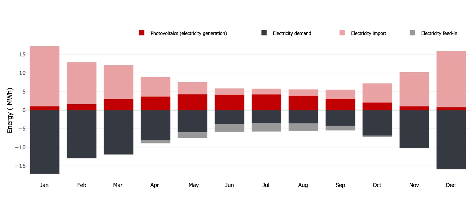
The geothermal borehole field is intended to provide heat and cooling for the 5GDHC network for the given district. The optimal PV module area is determined by the design optimization algorithm. The operation determined by the simulation is shown in Figures 8 and 9. The PV modules generate 32.7 MWh of electricity per year. This covers 28.5 % of the electricity demand in the district. The CO₂ emissions for this district are 28.7 tons per year.

Operational simulation of the energy system

Figure 8: The operational simulation shows the optimized energy system of geothermal boreholes including heat pumps and PV system

Figure 9: Electricity balance over the year

Step 5: Simulation of geothermal boreholes

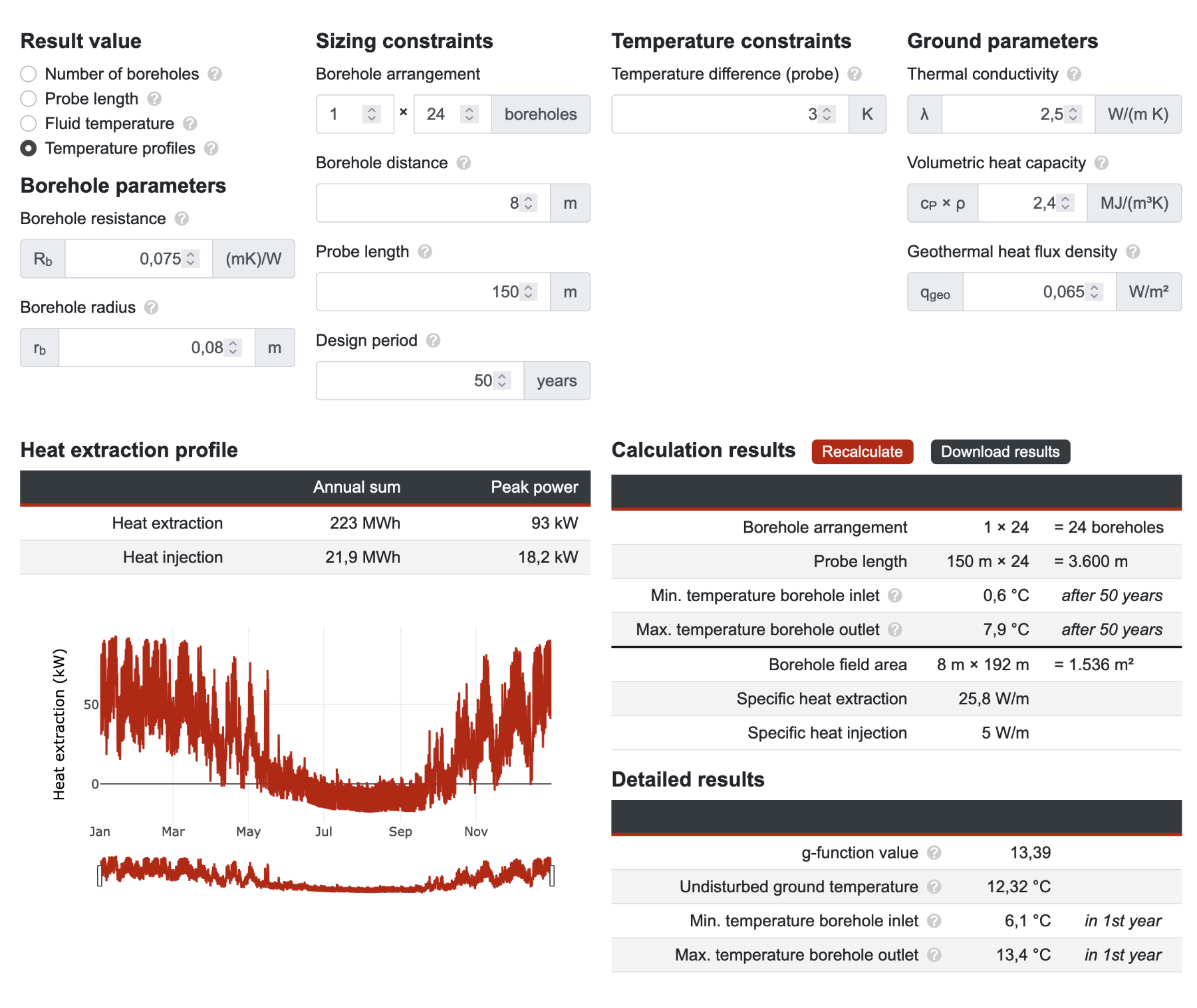
In the detailed design module for geothermal boreholes, precise information about the ground (e.g., thermal conductivity, volumetric heat capacity, heat flux density), the borehole (borehole resistance, borehole radius), and the design boundary conditions (e.g., borehole depth, borehole spacing) are defined, see Figure 10.

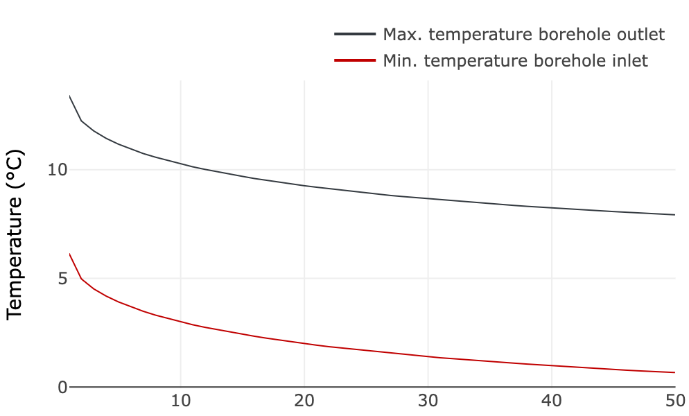
The calculation results show that 24 boreholes with:

25.8 W/m specific heat extraction
5 W/m specific heat injection

are sufficient to cover the heating and cooling demands of the district. The minimum temperature at the borehole inlet is 0.6 °C after 50 years for this borehole field configuration.

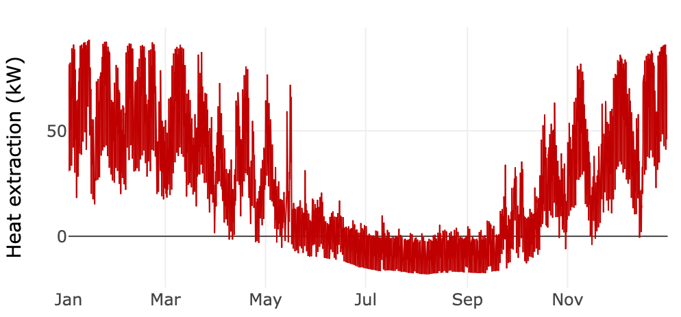
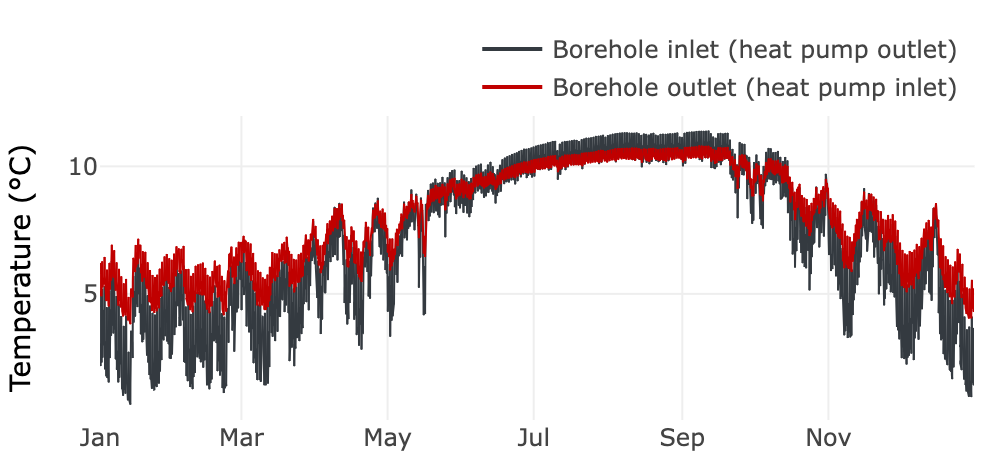
Figure 10: Design module for geothermal boreholes in nPro, simulation results for 24 boreholes

The simulation of the geothermal boreholes finally provides a detailed annual temperature profile for the borehole inlet (or heat pump outlet) and the borehole outlet (or heat pump inlet), see Figure 11.

Figure 11: Temperature profile at borehole inlet and outlet.

The heat balance can also be displayed over a longer period – e.g., 50 years – see Figure 12. In this case study, a temperature decrease over time can be observed, as the investigated energy system extracts more heat from the ground over the year than is returned through natural heat flow or active regeneration (e.g., passive cooling) in summer.

This annual heat extraction predominates, causing the ground to cool in the long term. A balanced heat balance and thus long-term efficiency of the heat pumps can be ensured through:

an optimized system design,
enforced heat reinjection (e.g., through passive cooling or solar thermal energy),
regular monitoring of heat extraction and reinjection rates.

Figure 12: Temperature profile over 50 years: maximum temperatures decrease over time as less heat is re-injected in summer than extracted over the year.

Step 6: Economic evaluation

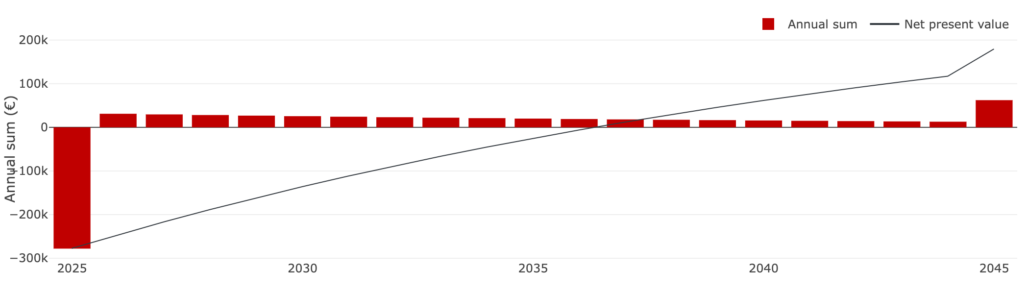
With nPro, the economic efficiency of the energy system with a 5GDHC network can be evaluated. Figure 13 shows the economic analysis.

The annual cash flow consists of the annual net expenses for the energy system, see Figure 13, including:

Investments (e.g., construction of the 5GDHC network, acquisition of heat pumps),
Replacement investments (e.g., replacement of components after their lifespan),
Ongoing operating costs (e.g., maintenance, energy supply),
Other annual costs (e.g., taxes, fees).

The net present value shows the cumulative financial evaluation of the project over the years. It considers:

Initial investments,
annual costs, and
future savings or revenues, discounted over the evaluation period.

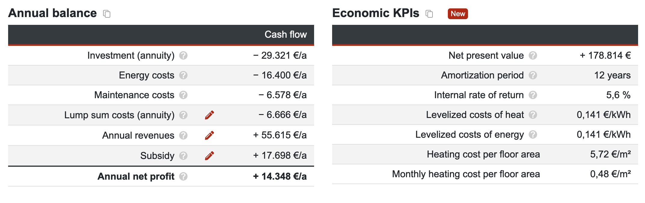
Figure 13: Economic evaluation in nPro

Under the Economic KPIs section in Figure 14, metrics such as the net present value at the end of the evaluation period (here the year 2045) and the payback period can be viewed.

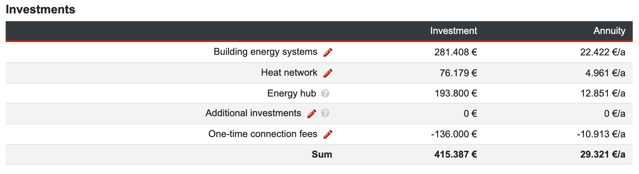
Economic evaluation: annual balance and key figures

Figure 14: The Annual balance and Economic KPIs sections summarize the economic evaluation, e.g., including investments, various operating costs, annual revenues, and the payback period.

In Figure 15, the individual listing of investments and one-time revenues (one-time connection fees) are outlined.

Figure 15: The investment section includes investments for building energy systems (decentralized heat pumps), the 5GDHC network, the energy center, other investments, and one-time revenues.

nPro enables a transparent evaluation of the profitability of the energy system through systematic analysis and visualization of all relevant costs, revenues, and long-term economic effects. This supports decision-makers in making informed investment decisions and ensuring the long-term profitability of the project.