Case study: Solar district heating with thermal storage

District

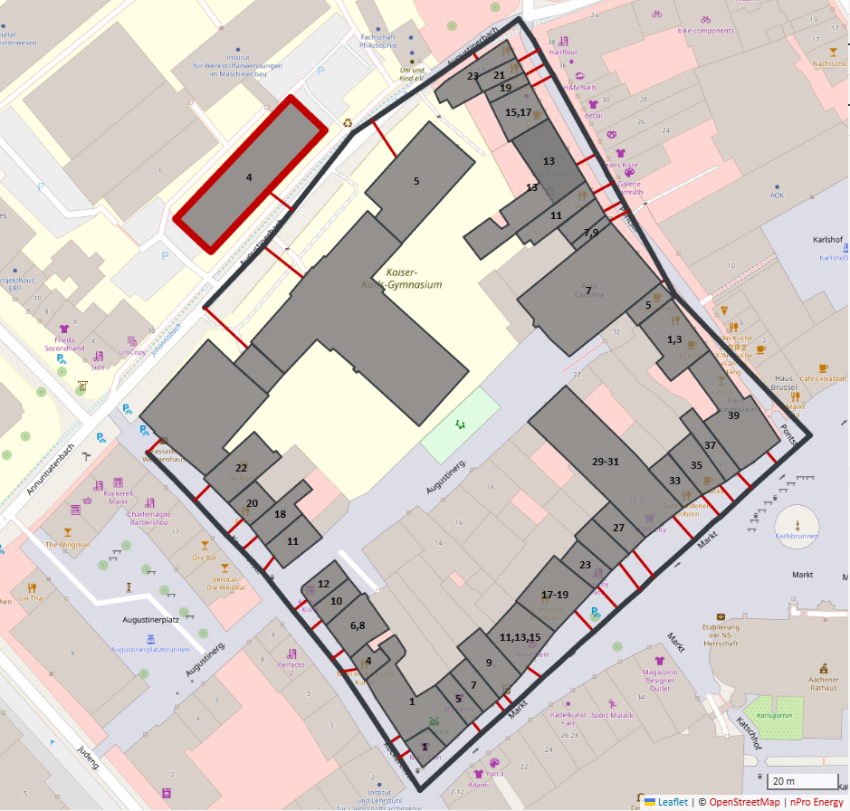
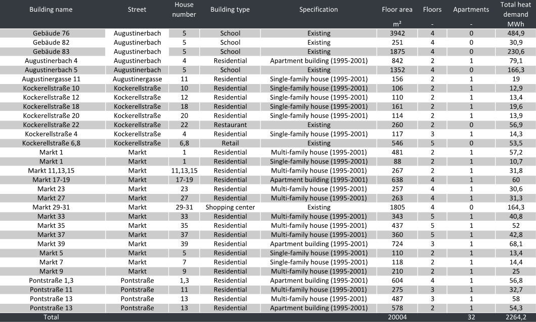
An energy supply system is planned for a sample district with 39 buildings. The district includes a school and several mixed-use residential buildings with retail spaces. The assumed location of the district is Aachen, Germany.

Figure 1: District with 39 buildings to be supplied. A building opposite the school is designated as the feed-in point.

Step 1: Demand analysis for heating, cooling and electricity

• Space heating and domestic hot water demand:
  • Covered via the heating network
• Cooling demand:
  • Supplied for space cooling and process cooling (e.g., server cooling) via a separate cooling network
• Electricity demand:
  • General demand for user electricity (e.g., for lighting)
  • Demand for e-mobility

Table 1: Building overview of the district to be supplied, exported as Excel from nPro (excerpt)

With nPro, demand profiles can be created with just a few clicks for each of the 39 buildings. Annual profiles with hourly resolution are crucial for district calculations, as time- and season-dependent renewable sources (here, solar thermal) are to be utilized.

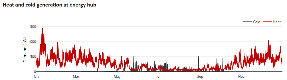
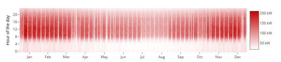
Step 2: Load profiles at the energy hub

After adding all buildings to the district, nPro can display the load profiles in hourly resolution. Figures 2 and 3 show the demand profiles at the energy hub for heating, cooling and electricity.

Figure 2: Heat and cooling demand profile at the energy hub. The temporarily increased cooling demand in summer is clearly visible (due to server room cooling in the school building).

Figure 3: Electricity demand: The heatmap shows lighter areas, indicating a lower electricity demand caused by the reduction in school electricity consumption during school holidays: Easter (late March to April), summer (July to mid-August), autumn (October), Christmas (late December to early January).

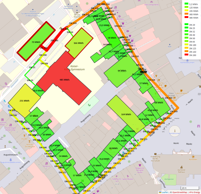
Step 3: Pipe sizing

In nPro, pipe diameters for heating networks can be automatically sized and mapped visually. The nominal diameter of the pipes is determined based on the heat demand of the buildings and the heat losses in the network. The pipe sizing is shown in Figure 4.

Figure 4: In nPro, various attributes of the buildings and the heating network can be displayed cartographically, e.g., the total heat demand of each building and the nominal diameter of individual pipe sections.

Step 4: Energy hub design

For this district, a heating and cooling supply, as well as an electricity supply, will be implemented using solar thermal energy.

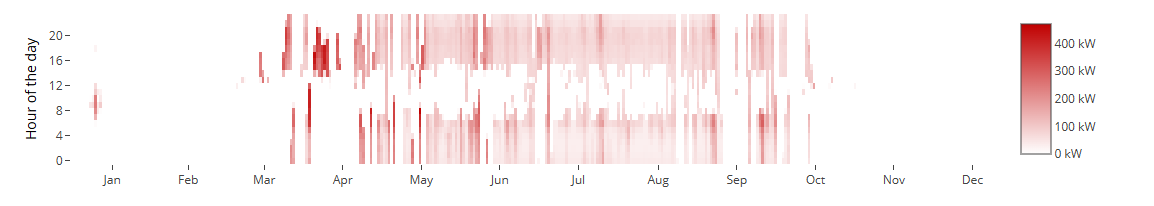
A connection to an existing district heating network is assumed at the energy hub for baseload coverage. Heat from the solar thermal system is used directly in the district, while surplus heat can be fed into the district heating network. The solar thermal heat generation is shown in Figures 5a and 5b for the following azimuth angles:

• 60° (azimuth) with 103 kWh/m² yield per collector area
• 15° (azimuth) with 163 kWh/m² yield per collector area

Figure 5a: Heat generation using solar thermal (60° azimuth) over the course of the year.

Figure 5b: Heat generation using solar thermal (15° azimuth) over the course of the year.

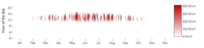
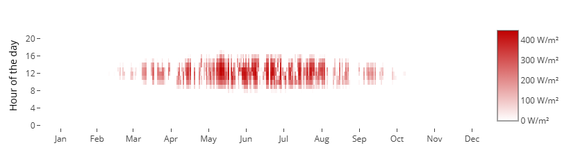
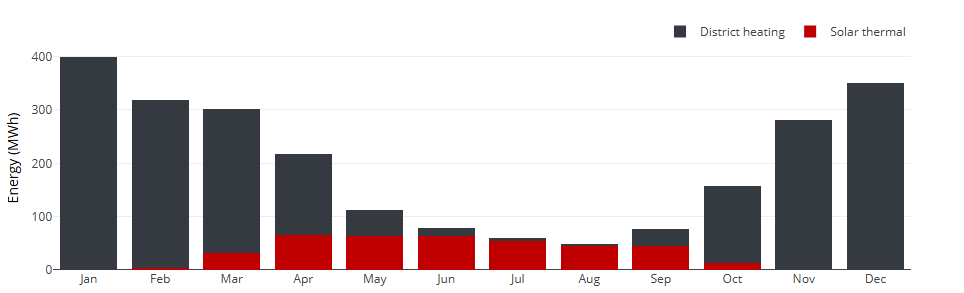
Figure 6 shows the operation of the optimized energy supply system by nPro. Cooling loads are met using compression chillers. The specified solar thermal area is 3,000 m², which is the maximum installable area for this district. The solar thermal system produces 247 kWh of heat per m² of collector area annually, totaling 307 MWh. Thus, 15.9% of the district’s heat demand is covered by the solar thermal system, while the remaining 84.1% is covered by the external district heating connection. The electricity required for buildings and compression chillers is drawn directly from the power grid.

Figure 6: Optimized energy system with solar thermal system and thermal storage.

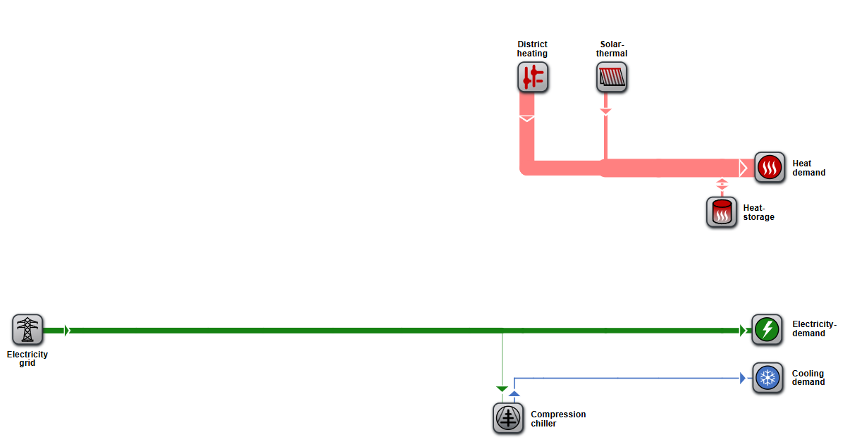
Figure 7 shows the heat supply from the external district heating network. It can be observed that in summer, almost no heat needs to be drawn from the external district heating network due to the solar thermal system and the thermal storage.

Figure 7: Heat supply from both sources throughout the year. Due to the solar thermal system, almost no heat needs to be imported from the external district heating network in summer.

The operation of the thermal storage (Figure 8) shows that the storage is charged in the afternoon hours during summer and discharged during evening/night hours.

Figure 8: Operation of the thermal storage (discharing power): The storage is primarily used in summer to utilize excess heat from the solar thermal system during the evening and nighttime.

Step 5: Economic analysis

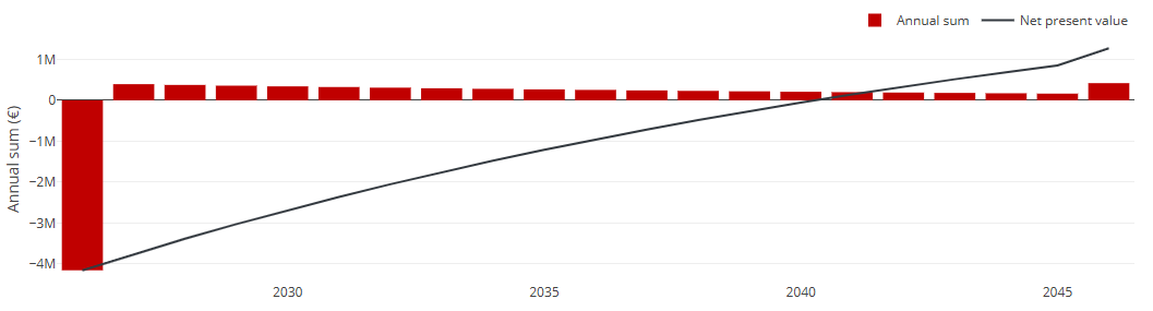
nPro enables an economic analysis of the energy supply system. Figure 9 shows the development of the net present value over the system's lifetime. A positive net present value at the end of the project duration indicates that the investment is economically viable. The ecological analysis in nPro also shows that CO₂ emissions for this district amount to 563 t per year.

Figure 9: Economic viability visualized through net present value development. The payback period here is 15 years.

In nPro, various optimization targets can be selected for automatic system sizing:

• Net present value / annualized total costs
• Multi-objective optimization: net present value and CO₂ emissions
• CO₂ emissions
• Minimal electricity purchase from the grid (maximum self-sufficiency)

In this case study, net present value was chosen as the optimization target.

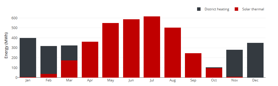
An optimization based on CO₂ emissions would, for example, lead to a significant enlargement of the solar thermal system - up to the maximum set value of 10,000 m². This would significantly increase the share of heat covered by solar thermal over the year. This is clearly visible in Figure 10 compared to Figure 7:

Figure 10: Heat supply from both sources throughout the year. In this theoretical case, with a total collector area of 10,000 m², the heat demand from April to September could be fully covered by solar thermal.

Video tutorials

Extensive video tutorials on calculating districts and heating networks in nPro can be found here: nPro tutorials

This might also interest you

• All features of nPro
• Case study: Hydrogen district
• 5GDHC (anergy) networks