

This page describes the economic feasibility analysis in nPro using an example district project with a heating network. You will not only see the result, but every single item along the way – from the investment to the net present value after 20 years.
Fundamentals of the economic feasibility analysis
The economic analysis in nPro is based on the VDI guideline 2067 (Economic efficiency of building installations – Fundamentals and economic calculation). Adopted from the guideline are, in particular, the annualization of investments via a discount rate and the technical service life, the consideration of replacement investments and residual values, as well as the approach of treating maintenance costs as a percentage of the investment. All investments for the building energy systems, the heating network and the central components in the energy center are taken into account – i.e. the district as a whole and not just individual plants.
The calculation is carried out from the perspective of the operator of the energy system: what the building owners pay for delivered heat, cooling and electricity appears as revenue. It is therefore a business-economic and not a macroeconomic view of the district.
Annuities and net present value
Investments occur once, but their benefit is spread over many years. To make both comparable, the investments are converted into annuities via the discount rate and the technical service life of the respective technology, i.e. into uniform annual payments. Together with all ongoing costs and revenues, they yield the total annual costs and revenues.
The net present value and the annual balance are thus two representations of the same thing: because the annual balance already contains the annualized investments, lump-sum costs and subsidies, its balance corresponds exactly to the annuity of the net present value. A positive balance consequently also means a positive net present value – and therefore a project that is economically viable under the chosen assumptions.
Decisive for this conclusion is that the initial investment is included in the annual balance. It could not be drawn from the ongoing cash inflows and outflows alone: a project can generate ongoing surpluses and still show a negative net present value because of high initial investments.
The revenues also include the operator’s income received from the building owners for the heating, cooling and electricity demands covered. In nPro, these can be modelled via energy prices (€/kWh), capacity prices (€/kW) and base prices (€/year) – i.e. exactly the way heat supply contracts are structured in practice.
Residual values and replacement investments
The technical service life of a plant rarely matches the project duration exactly. In accordance with VDI 2067, nPro covers both cases:
- Residual values: if the technical service life is longer than the period under consideration – for example with a heating network with a service life of 40 years and a project duration of 20 years – a residual value remains at the end, which is applied as revenue in the final year and discounted. Depreciation is linear over the service life.
- Replacement investments: if the service life is shorter than the period under consideration, the plant must be replaced during the project duration. The replacement investment is booked at the corresponding point in time and discounted.
Particularly in district projects, this makes a considerable difference: otherwise the long-lived heating network and the short-lived battery would be measured by the same yardstick.
Which payments are taken into account
The one-off payments include:
- investments for the plants (building energy system, heating network and energy center),
- subsidies on investments (reported separately, not part of the investments), and
- lump-sum costs (reported separately, not part of the investments).
In addition, annual costs are included in the calculation:
- energy costs (e.g. for electricity purchase),
- maintenance costs (specified as a percentage of the investment),
- revenues (e.g. for electricity feed-in or for covering the heating demand),
- CO2 costs, and
- other operating costs (e.g. insurance and administrative costs).
In the case example, these payments are assumed to be nominally constant, i.e. no price increase is assumed. For the net present value calculation, they are discounted to year 0. Annual rates of price change – for example for electricity, fuels, the CO2 price or heat revenues – can be entered in the general economic settings and considerably influence the result over 20 years; a comparison with and without price increases is therefore worthwhile in almost every project.
As a result, the calculation provides various economic key figures with which the profitability of a project can be assessed:
- Net present value: the sum of all cash flows over the time horizon considered, discounted to year 0.
- Internal rate of return: the discount rate at which the net present value becomes exactly zero.
- Payback period: the point in time at which the cumulative, discounted cash flow first becomes positive – i.e. a dynamic payback that includes the interest effect. If the net present value remains negative over the entire duration, as in the case example below, no such point in time exists and no payback period is reported.
Description of the example district
The economic feasibility analysis is explained below using an example district. First, the district and the input variables of the simulation are described. All values are freely chosen assumptions of this case example.
Project data
The discount rate (here 5 %) and the time horizon considered (here 20 years) are defined in the project data. The supply solution is a cold district heating network (anergy network) with decentralized heat pumps, which also provides the cooling supply. A subsidy on the investments for the building energy systems, the heating network and the plants in the energy center is taken into account.
In addition, other costs can be defined – for items that cannot be captured anywhere else in the calculation. Both other investment costs (one-off, e.g. land or connection costs) and other operating costs (annual, e.g. insurance) are possible.
Buildings
Three different building energy systems are considered in the district:
- Network heat pump: it uses the heating network as a heat source and covers the heating demands that cannot be covered directly from the heating network because the network temperatures are too low. The cooling demand is covered by passive cooling with the heating network.
- Ground-source heat pump: it covers the building’s heating demands; the peak load is handled by an electric heating element. Waste heat from the cooling supply is not fed into the heating network.
- Air-source heat pump: it covers the building’s heating demands, with the peak load again handled by an electric heating element. The cooling demand is covered entirely by an air-cooled chiller with a dry cooler, whose waste heat is released to the ambient air.

Heating network
The heating network for the 30 buildings is 800 m long. For simplicity, the costs are applied as lump sums of 500 €/m for the pipe network and 400 €/m for the excavation work. The pipe network costs are incurred twice per trench meter (supply and return), the excavation work only once. A technical service life of 40 years and maintenance costs of 1 % of the investment are assumed. Since the time horizon considered is only 20 years, the heating network still has a residual value at the end of it, which is depreciated linearly and discounted.
Energy center
The energy center comprises all technologies that are not installed in the buildings – here photovoltaics, a biomass boiler, solar thermal collectors, air-source heat pumps, geothermal probes and batteries. A minimum area of 400 m2 is specified for the solar thermal system and a minimum storage capacity of 50 kWh for the battery. The energy price for electricity is 0.3 €/kWh, that for biomass 0.045 €/kWh; CO2 pricing is set at 100 €/tCO2.
Economic feasibility: evaluation
The results of the economic feasibility analysis for the district project are explained in detail below.
Annual balance
The annual balance provides a first overview by relating all costs, subsidies and revenues to one year. Investments, lump-sum costs and subsidies appear in it as annuities. This is an annualized representation and not an actual payment: in fact, these amounts are incurred once in year 0; the annuity distributes them evenly over the time horizon considered for calculation purposes, so that they become comparable with the ongoing costs and revenues.
The balance contains the annuities of the initial investments of all generation and storage technologies including user-defined additional investments, the energy costs (electricity, natural gas, biomass and others), the total maintenance and operating costs, as well as the costs of CO2 pricing as the product of the CO2 price and the emissions.
On the revenue side are the income from energy feed-in – for example into the electricity grid – and from covering the energy demands for heating, cooling, electricity and hydrogen. The balance of all annual costs and revenues concludes the annual balance: a positive value means an annual surplus, a negative one a deficit. Additional key figures can also be reported, for example the surplus per floor area.
| Annual payment | |
|---|---|
| Investment (annuity) | - 544,700 €/a |
| Energy costs | - 61,597 €/a |
| Maintenance costs | - 59,954 €/a |
| CO2 costs | - 13,303 €/a |
| Lump-sum costs (annuity) | - 294,803 €/a |
| Revenues | + 231,527 €/a |
| Subsidy | + 53,154 €/a |
| Annual surplus | - 689,675 €/a |
| Surplus per floor area | - 52 €/m² |
In the case example, the balance is clearly negative at around -690,000 €/a. The two largest items are the annuities of the investments and of the lump-sum costs – a typical picture for district projects in which extensive refurbishment measures are part of the concept.

Net present value
The net present value table shows the cash inflows and outflows over the entire project period, separated into investments, annual costs and annual revenues.
All values in the table are already discounted to year 0. The nominally constant annual costs of 134,854 €/a therefore appear in year 1 as 128,432 € (134,854 € / 1.05), in year 2 as 122,316 € and so on; the revenues accordingly. The net present value is therefore the simple cumulation of the annual totals and requires no further discounting.
At the start of the project in year 0, investments and lump-sum costs are incurred, against which the subsidy is offset: 8,164,210 € + 3,673,894 € - 662,421 € = 11,175,683 €.
Two further investments appear during the project duration: the -23,387 € in year 11 is the discounted replacement investment for the battery, which reaches its technical service life before the end of the time horizon considered; the -6,682 € in year 16 is, accordingly, the replacement investment for the air-source heat pump of the building energy systems, which has a service life of 15 years.
The positive amount of 1,406,112 € in year 20 describes the residual values of all those plants that have not yet reached their technical service life at the end of the time horizon considered – for example the heating network with a service life of 40 years. Linear depreciation is assumed.
| Year | Investment | Annual costs | Annual revenues | Annual total | Net present value |
|---|---|---|---|---|---|
| 0 | -11,175,683 € | 0 € | 0 € | -11,175,683 € | -11,175,683 € |
| 1 | 0 € | -128,432 € | 220,502 € | 92,070 € | -11,083,613 € |
| 2 | 0 € | -122,316 € | 210,002 € | 87,685 € | -10,995,928 € |
| 3 | 0 € | -116,492 € | 200,002 € | 83,510 € | -10,912,418 € |
| 4 | 0 € | -110,944 € | 190,478 € | 79,533 € | -10,832,885 € |
| 5 | 0 € | -105,661 € | 181,407 € | 75,746 € | -10,757,139 € |
| 6 | 0 € | -100,630 € | 172,769 € | 72,139 € | -10,685,000 € |
| 7 | 0 € | -95,838 € | 164,542 € | 68,704 € | -10,616,296 € |
| 8 | 0 € | -91,274 € | 156,706 € | 65,432 € | -10,550,864 € |
| 9 | 0 € | -86,928 € | 149,244 € | 62,316 € | -10,488,548 € |
| 10 | 0 € | -82,788 € | 142,137 € | 59,349 € | -10,429,199 € |
| 11 | -23,387 € | -78,846 € | 135,369 € | 33,136 € | -10,396,063 € |
| 12 | 0 € | -75,092 € | 128,923 € | 53,831 € | -10,342,232 € |
| 13 | 0 € | -71,516 € | 122,784 € | 51,268 € | -10,290,964 € |
| 14 | 0 € | -68,110 € | 116,937 € | 48,827 € | -10,242,137 € |
| 15 | 0 € | -64,867 € | 111,368 € | 46,501 € | -10,195,636 € |
| 16 | -6,682 € | -61,778 € | 106,065 € | 37,606 € | -10,158,030 € |
| 17 | 0 € | -58,836 € | 101,014 € | 42,178 € | -10,115,852 € |
| 18 | 0 € | -56,034 € | 96,204 € | 40,170 € | -10,075,682 € |
| 19 | 0 € | -53,366 € | 91,623 € | 38,257 € | -10,037,425 € |
| 20 | 1,406,112 € | -50,825 € | 87,260 € | 1,442,547 € | -8,594,878 € |
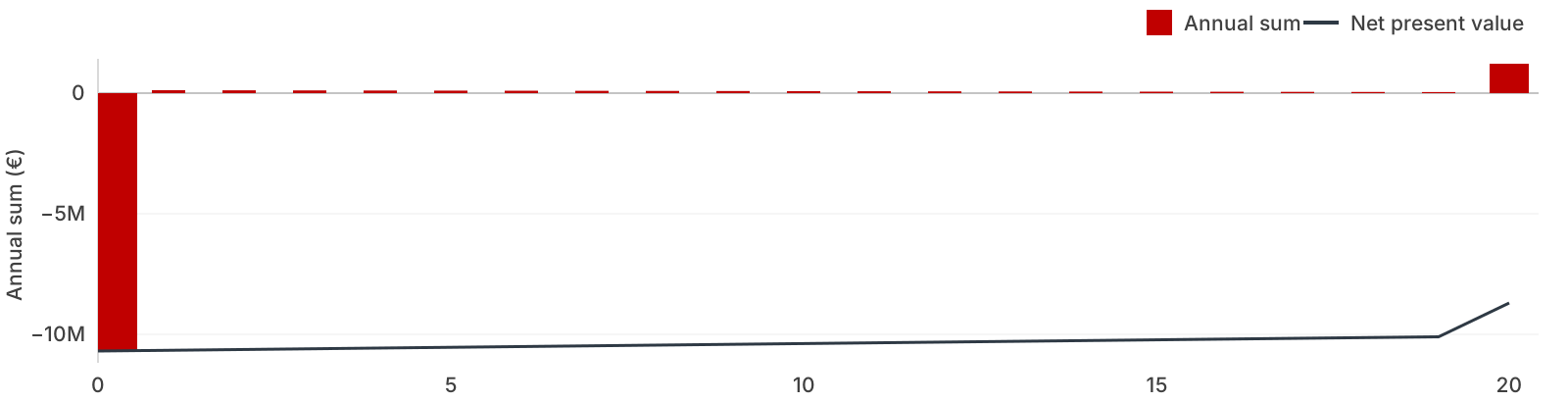
Both evaluations can be converted into one another: with the annuity factor for 5 % and 20 years (0.0802), the net present value of -8,594,878 € yields exactly the annual surplus of around -689,675 €/a from the annual balance. The net present value and the annual balance therefore describe the same result, once as a total sum and once as an annual value.
Breakdown of costs and revenues
The individual items of the cost and revenue breakdown are described in detail below.
Investments
The building energy systems category comprises the investments for all generation and storage plants in the buildings, presented as annuities; in the case example these amount to 1,137,960 € with an annuity of 86,552 €/a. Replacement investments are taken into account here.
Refurbishment measures such as additional insulation of the building envelope or measures to lower the supply temperature are reported separately – here 4,400,000 € with an annuity of 273,227 €/a. The heating network costs comprise trench and pipe costs and can be freely defined by the user. Further investments are incurred for all plants in the energy center (1,006,250 €, annuity 71,864 €/a). The user-defined other investments amount to 500,000 € with an annuity of 40,121 €/a; the project duration is used to annualize them.
In total, the investments amount to 8,164,210 € with an overall annuity of 544,700 €/a.
| Investment | Annuity | |
|---|---|---|
| Building energy systems | 1,137,960 € | 86,552 €/a |
| Refurbishment measures | 4,400,000 € | 273,227 €/a |
| Heating network | 1,120,000 € | 72,936 €/a |
| Energy center | 1,006,250 € | 71,864 €/a |
| Other investments | 500,000 € | 40,121 €/a |
| Total | 8,164,210 € | 544,700 €/a |
Energy costs
The following table shows how the energy costs are split up. The electricity costs relate to the electricity purchase of the energy center. The operating electricity for heat pumps or electric heating elements in the buildings and the pumping electricity for the heating network are not purchased via the energy center in this case example, but directly from the electricity grid, and are therefore applied with a separate energy price. The breakdown is supplemented by further energy carriers, here biomass.
| Price | Energy amount | Costs | |||
|---|---|---|---|---|---|
| Electricity purchase (energy center) | 0.3 €/kWh | x | 76 MWh/a | = | 22,800 €/a |
| Biomass | 0.045 €/kWh | x | 73 MWh/a | = | 3,285 €/a |
| Purchase of operating electricity from the grid | 0.12 €/kWh | x | 279 MWh/a | = | 33,457 €/a |
| Purchase of pumping electricity from the grid | 0.12 €/kWh | x | 17.1 MWh/a | = | 2,055 €/a |
| Total | 61,597 €/a |
Maintenance costs
The maintenance costs are reported separately for the three system parts building energy systems, heating network and energy center. In addition, there are further annual operating costs such as base prices or insurance.
| Costs | |
|---|---|
| Building energy systems | 18,746 €/a |
| Heating network | 11,200 €/a |
| Energy center | 25,008 €/a |
| Other operating costs | 5,000 €/a |
| Total | 59,954 €/a |
CO2 costs
The CO2 costs result from the annual equivalent emissions and the CO2 price entered.
| Price | Annual emissions | Costs | |||
|---|---|---|---|---|---|
| CO2 costs | 100 €/t | x | 133 t/a | = | 13,303 €/a |
Lump-sum costs
The lump-sum costs represent those items that, in practice, can be calculated as a percentage of the project costs: planning services, for example by engineering firms, delivery, installation and commissioning of the plant technology, measurement and control technology as well as a surcharge for unforeseen additional costs. All percentages can be freely defined.
In this case example, the reference value is the entire investment sum including the refurbishment measures. At a combined 45 %, this results in lump-sum costs of 3,673,894 € with an annuity of 294,803 €/a – an amount of the same order of magnitude as the refurbishment itself and therefore a key lever for the overall result.
| Investments | Percentage | Costs | |||
|---|---|---|---|---|---|
| Planning costs | 8,164,209 € | x | 10 % | = | 816,421 € |
| Delivery, installation, commissioning | 8,164,209 € | x | 10 % | = | 816,421 € |
| Measurement and control technology | 8,164,209 € | x | 15 % | = | 1,224,631 € |
| Unforeseen costs | 8,164,209 € | x | 10 % | = | 816,421 € |
| Total | 3,673,894 € | ||||
| Annuity | 294,803 €/a |
Revenues
In the case example, the revenues consist of the electricity feed-in as well as the revenues for the heating and cooling demand covered in the buildings. For heating and cooling, a distinction is made in each case between the energy price, capacity price and base price – this allows real price sheets to be reproduced. The specific conditions are agreed between the operator and the customers in practice. In total, this results in 231,527 €/a.
| Remuneration | Amount | Revenues | |||
|---|---|---|---|---|---|
| Electricity feed-in | 0.04 €/kWh | x | 37.4 MWh/a | = | 1,496 €/a |
| Heating demand | 0.12 €/kWh | x | 1,030 MWh/a | = | 123,648 €/a |
| Heating demand (capacity price) | 50 €/kW/a | x | 673 kW | = | 33,652 €/a |
| Heating demand (base price) | 200 €/bldg. | x | 30 bldg. | = | 6,000 €/a |
| Cooling demand | 0.1 €/kWh | x | 264 MWh/a | = | 26,400 €/a |
| Cooling demand (capacity price) | 50 €/kW/a | x | 687 kW | = | 34,331 €/a |
| Cooling demand (base price) | 200 €/bldg. | x | 30 bldg. | = | 6,000 €/a |
| Total | 231,527 €/a |
Subsidy
Subsidies can be applied as flat-rate subsidy rates to three investment blocks: to the building energy systems (e.g. heat pumps or chillers), to the heating network (pipes and installation costs) as well as to the plants in the energy center (e.g. large-scale heat pump or thermal storage). The subsidy reduces the investment in year 0; for the annual balance it is annualized in the same way as the investments.
| Subsidy rate | Investment | Subsidy | ||
|---|---|---|---|---|
| Building energy systems | 10 % | 1,137,960 € | 113,796 € | |
| Heating network | 40 % | 1,120,000 € | 448,000 € | |
| Energy center | 10 % | 1,006,250 € | 100,625 € | |
| Total | 662,421 € | |||
| Annuity | 53,154 €/a |
Investments: detailed listing
The following sections show the investments of the three system parts in detail, in each case with the number of components, investment costs, annual annuity and annual maintenance costs. Depreciation is over the user-defined technical service life; the annuity results from the investment sum, the depreciation period and the discount rate. In accordance with VDI 2067, the maintenance costs are applied as a percentage of the investment costs.
Investments in the buildings
The table lists all components of the building energy systems. In the example, 26 network heat pumps are installed, each of which requires its own connection to the heating network.
| Number | Investment | Annuity | Maintenance | |
|---|---|---|---|---|
| Heating network connection | 26 | 229,235 € | 14,928 €/a | 2,292 €/a |
| Network heat pump | 26 | 748,400 € | 60,054 €/a | 14,968 €/a |
| Ground-source heat pump | 2 | 12,585 € | 1,010 €/a | 252 €/a |
| Air-source heat pump | 2 | 14,585 € | 1,412 €/a | 292 €/a |
| Geothermal probes | 2 | 81,940 € | 5,088 €/a | 0 €/a |
| Electric heating element | 4 | 8,245 € | 612 €/a | 82 €/a |
| Air-cooled chiller | 2 | 42,970 € | 3,448 €/a | 859 €/a |
| Refurbishment measures | --- | 4,400,000 € | 273,227 €/a | --- |
| Total | 64 | 5,537,960 € | 359,779 €/a | 18,746 €/a |
Investments in the heating network
The investment and maintenance costs of the heating network result from its length.
| Length | Investment | Annuity | Maintenance |
|---|---|---|---|
| 0.8 km | 1,120,000 € | 72,936 €/a | 11,200 €/a |
Investments in the energy center
The table contains all components of the energy center with the associated investments and maintenance costs.
| Investment | Annuity | Maintenance costs | |
|---|---|---|---|
| Photovoltaics | 61,600 € | 4,943 €/a | 616 €/a |
| Biomass boiler | 2,250 € | 181 €/a | 68 €/a |
| Solar thermal | 160,000 € | 12,839 €/a | 2,400 €/a |
| Air-source heat pump | 149,600 € | 12,004 €/a | 3,740 €/a |
| Geothermal probes | 592,800 € | 36,811 €/a | 17,784 €/a |
| Battery | 40,000 € | 5,086 €/a | 400 €/a |
| Total | 1,006,250 € | 71,864 €/a | 25,008 €/a |
From the result to an economically viable variant
The case example ends with a negative net present value – a result that is completely normal in early project phases. What matters is what follows from it: the detailed breakdown shows exactly which items drive the result, and thus also which levers can be adjusted. In the present case, the annuities of the investments and of the lump-sum costs are the dominant block, at around 840,000 €/a combined.
Typical starting points for a revision are:
- Extent of the refurbishment measures: at 4.4 million €, they represent the largest single item. A smaller scope of refurbishment directly reduces the investments, but increases the heating demands – a conflict of objectives that only a recalculation can resolve.
- Revenue model: energy, capacity and base prices for heating and cooling can be varied separately in order to find a viable price sheet.
- Subsidy rates: higher subsidy rates, for example for the heating network, act directly on the investment in year 0.
- Design of the energy center: using the optimization model, technologies and capacities can be redetermined in a cost-optimal way instead of specifying a configuration.
- Network concept: trench length and connection density substantially determine the network costs per kilowatt-hour delivered (see linear heat density).
- Discount rate and time horizon: both considerably influence the annuities and should match the financing situation of the project.
- Price development: constant prices are assumed in the case example. If rates of price change are entered for electricity, fuels, CO2 and heat revenues, the result shifts significantly over 20 years – usually in favor of the systems with low fuel demand.
Because each of these changes only requires a recalculation in nPro, variants can be calculated in quick succession and compared directly – until a configuration is found that works both technically and economically.