Pressure calculation in district heating networks
In nPro, absolute pressures in supply and return lines of a district heating network are calculated based on pipe losses, geodetic height differences and pressure losses at transfer stations and fittings. This calculation ensures that sufficient pressure is maintained throughout the entire network to avoid cavitation and to comply with hydraulic boundary conditions.
Calculation Principle
The pressure calculation is based on pressure losses in pipes and geodetic height differences in the network. Starting point is the minimum pressure at the energy center, which is specified by the user as a boundary condition in hydraulic settings. First, pressure losses along pipes (Pa/m) are determined during network design. Subsequently, a linear system of equations is set up to calculate nodal pressures throughout the entire network.
Calculation of Nodal Pressures
For each pipe, an equation is formulated that describes the pressure difference between connected nodes. The resulting system of equations is then solved numerically.
Pressure Components Considered in Network Simulation
Pipe Pressure Losses
The pressure losses (in Pa) in pipes are derived from hydraulic losses calculated during the design process.
Geodetic Pressure Differences
Height differences in the network lead to static pressure changes. These are calculated using the hydrostatic equation:
$$\Delta p = \rho \cdot g \cdot \Delta h$$
Where \( \rho \) is fluid density, \( g \) is gravitational acceleration, and \( \Delta h \) is the height difference between two points in the network. Pressure difference between two points can accordingly be expressed as:
$$p_2 = p_1 + \rho \cdot g \cdot (h_1 - h_2)$$
Neglection of Dynamic Pressure
In pressure calculation, dynamic pressure is neglected, as in heating networks it is typically very small compared to static pressure differences caused by height differences and pipe friction losses. Dynamic pressure results from flow velocity of the fluid and is generally given by:
$$p_\text{dyn} = \frac{1}{2} \cdot \rho \cdot v^2$$
Minimum Pressure and Safety Margins
For safe operation of a heating network, pressure throughout the entire network must remain above vapor pressure of the heat transfer medium. If vapor pressure is locally undercut, formation of vapor bubbles (cavitation) can occur, which may lead to unstable operation and damage to system components. High points in the network are particularly critical, as static pressure is lowest at these locations due to geodetic height differences. Therefore, it is verified whether minimum pressure in the network exceeds a defined safety threshold. The minimum pressure requirement is derived from vapor pressure of the heat transfer medium at maximum network temperature plus additional safety margins:
$$p_\text{min} = \frac{p_\text{vapor}(T_\text{max})}{10^5} + \Delta p_\text{hp} + \Delta p_\text{gen}$$
Where \(p_\text{vapor}(T_\text{max})\) denotes vapor pressure of the heat transfer medium at maximum network temperature \(T_\text{max}\). The following safety margins are considered:
- \(\Delta p_\text{hp} = 0.5\) bar: safety margin at the highest network point to prevent cavitation
- \(\Delta p_\text{gen} = 1.0\) bar: general safety margin to account for operational and model uncertainties
Calculation of Vapor Pressure (Antoine Equation)
The vapor pressure of the heat transfer medium is calculated as a function of temperature using the Antoine equation. This equation describes the relationship between temperature and saturation vapor pressure of a substance and is commonly used to determine vapor pressure of water.
$$\log_{10}(p_\text{mmHg}) = A - \frac{B}{C + T}$$
Where \(T\) is temperature in °C and \(A\), \(B\) and \(C\) are substance-specific Antoine coefficients. This equation initially yields vapor pressure in mmHg. A subsequent conversion to Pascal is performed:
$$p_\text{vapor} = p_\text{mmHg} \cdot 133.322$$
For water, the following coefficient ranges are used:
| Temperature range | A | B | C |
|---|---|---|---|
| 1 – 100 °C | 8.07131 | 1730.63 | 233.426 |
| 100 – 374 °C | 8.14019 | 1810.94 | 244.485 |
Data Source for Elevation Data
Geodetic heights of network components are automatically derived from digital elevation models (DEM). Copernicus DEM-90 elevation data is used as data basis, providing near-global coverage with a spatial resolution of approximately 90 m. These datasets enable consistent and automated determination of terrain topography across the entire network area. Data is automatically enriched during calculation for pipes with an undefined geodetic height or a height of 0 m.
| Region | Latitude (°N) | Longitude (°E) | Resolution |
|---|---|---|---|
| Central Europe | 43.0 – 58.0 | −9.4 – 25.0 | 90 m |
| Scandinavia | 53.4 – 71.6 | 4.0 – 42.1 | 90 m |
| Northeastern United States | 36.5 – 47.5 | −89.9 – −69.8 | 90 m |
| U.S. West Coast | 32.1 – 50.0 | −124.8 – −114.5 | 90 m |
| Chile & Western Argentina | −56.1 – −22.7 | −76.0 – −64.5 | 90 m |
| Eastern China & Korea | 24.0 – 41.0 | 109.9 – 130.1 | 90 m |
| Southern Europe (Mediterranean) | 34.5 – 44.0 | −10.0 – 30.9 | 90 m |
Additional regions will be added in the future and can also be integrated into the terrain database upon request. For regions not currently covered, an elevation of 0 m is assumed in pressure calculation.
Calculation and Visualization of Pressure Profiles in nPro
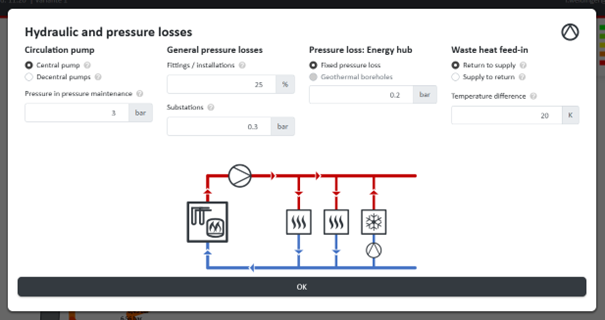
Hydraulic Settings
The hydraulic boundary conditions of the heating network can be adjusted on a project-specific basis in the hydraulic settings. A choice can be made between a central circulation pump and decentralized pumps at the substations. The setpoint for the pressure maintenance, referenced to the return pipe at the energy center, can be individually defined. Additionally, the pressure losses of pipe fittings, heat transfer stations and the energy hub can be configured separately in order to represent the hydraulic conditions of the network as realistically as possible.
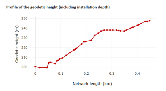
Visualization of Geodetic Heights
The elevation profile of all pipes can be displayed in the network visualization.
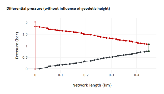
Visualization of Pressure Profiles
To analyze hydraulic conditions, the pressure profiles along the hydraulically most unfavorable path in the network are displayed (pipes from the energy hub to the critical point of the network). Both the pressures without consideration of geodetic height differences and the total pressures including the influence of topography are shown.
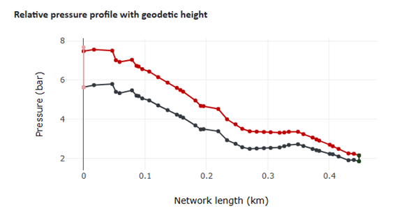
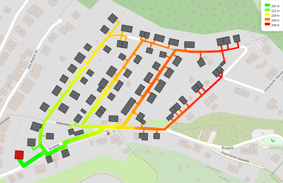
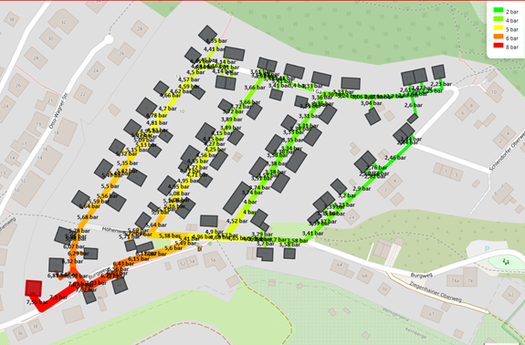
Furthermore, the absolute pressures of all pipes can be visualized on the map to analyze the pressure distribution across the entire network.
 English
 Deutsch


