Demand profile calculation: Validation for different building types
nPro makes it easy to generate hourly resolved demand profiles for space heating and air conditioning. On this page it is described how these are calculated and validated.
How are demand profiles calculated?
In nPro, a specially developed simplified calculation method is used to create demand profiles. This is essentially based on the degree-day method. It allows creating an hourly resolved demand profile based on a few input parameters. The special feature is that the energy reference area and the annual demand of the building as well as the peak load, if applicable, serve as input parameters. While these parameters are the actual results of detailed building simulations, for nPro, they are input values. This makes sense because in an early planning phase of a district only little information about the buildings is available. Often the building standard and floor area are known, but no detailed values of building physics, such as insulation thickness or degree of glazing. The annual energy demand can be estimated from the building standard and the peak load can also be derived with the help of full load hours. The simulation in nPro is thus used to generate profiles rather than to calculate the actual annual demand value. The advantage of this approach is that the profiles generated with nPro always satisfy the total annual demand and the peak loads defined by the user and, in addition, only very few input parameters are required. The annual profiles then represent a typical demand curve that can be expected for a building. For very special building types, such as a fully glazed office building, the profiles generated by nPro may differ from the profiles expected in reality.
How has the simulation method been validated?
Demand profiles generated with nPro have been validated for a variety of different buildings with different use types. For this purpose, free and open-source data from energy monitoring platforms of the city of Aachen [1] and the city of Frankfurt [2] was used. The monitoring data allow to analyze and download heat demand profiles in hourly resolution for more than one hundred buildings in Aachen and Frankfurt. An extract of the validation is provided in the following sections.
Heat demand of office and administration buildings
Office buildings have a comparatively low heating load due to high internal heat gains. Their profile is mainly characterized by strong differences between working days and weekend days. As an example, curves of the heat profile for 2 office buildings are shown below. Figure 1 shows the heat profile for a municipal administration building (Peterstraße 21-25, 52062 Aachen, Germany) for a period from 20.1. to 3.2.2018. The simulated heat demand profiles are shown in gray. The weekend on January 27 and 28 can be identified when only low heat demands occur. The daily peak loads are mostly well represented by the simulation. It is remarkable that on the first day (20.1.) the simulation shows only low heat demands (because it is a weekend day), whereas the real measured course resembles a normal working day. This could be, for example, due to the fact that there was a special event on that Saturday or that the heating control was programmed differently than on a normal weekend day due to another reason.
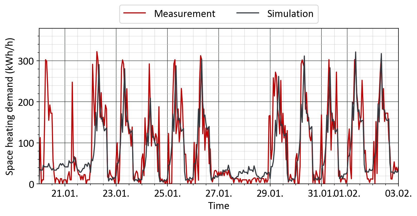
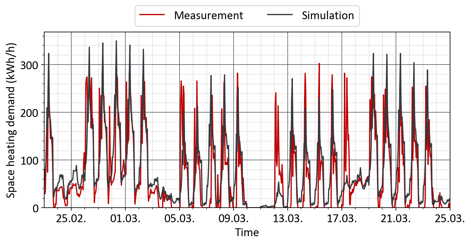
Figure 2 shows the heat demand profile of another public administration building (Markt 38-40, 52062 Aachen, Germany). The measured and simulated data are plotted for the period 23.2. to 25.3.2018. Once again, the weekends can be easily identified by the reduced heat demand. In the week of 25.2. the heat demands are highest, which is well represented by the simulation. The heating system runs continuously in this week, also during night and weekends, however, with lower output.
Heat demand of a public swimming pool
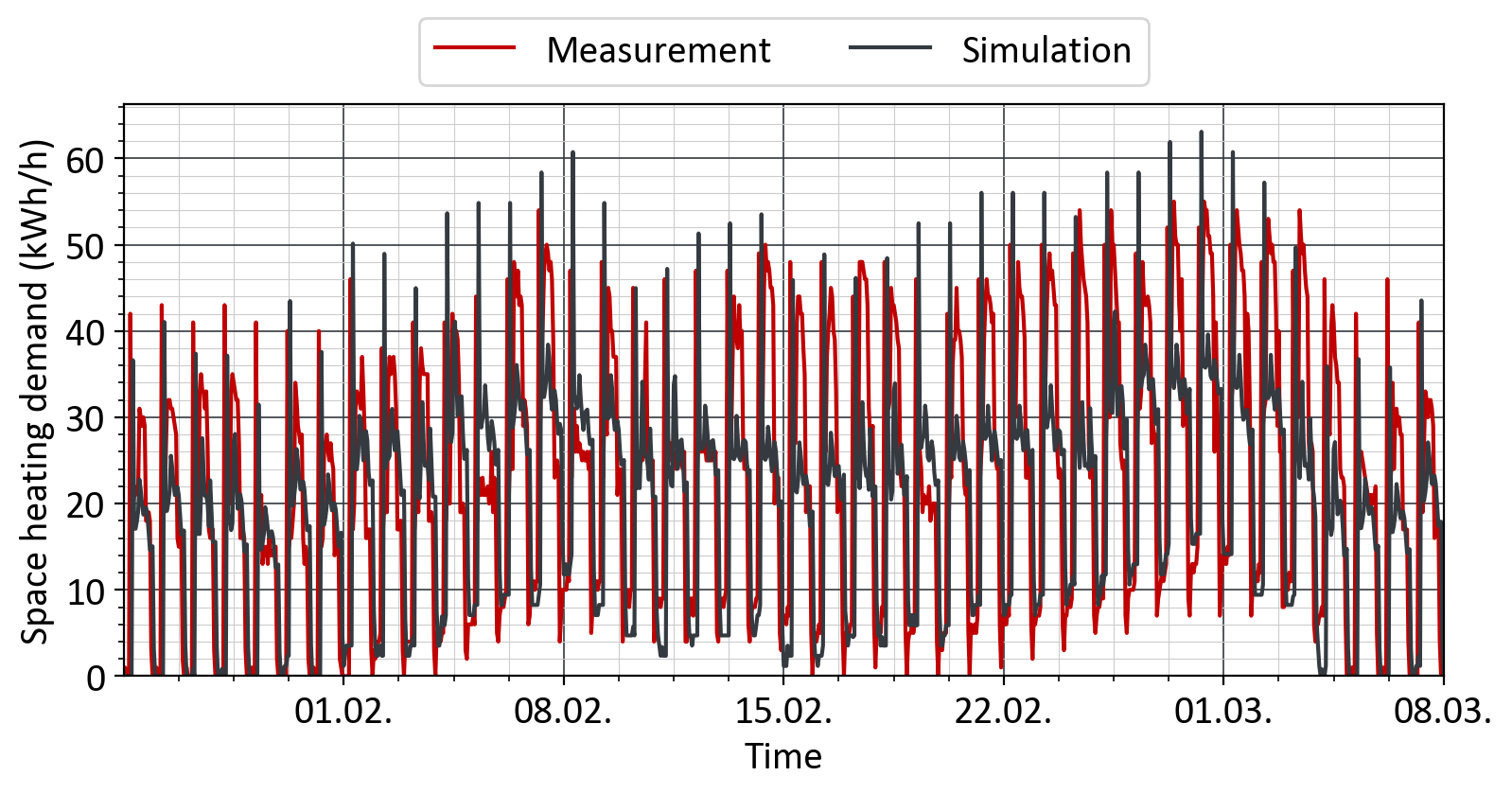
Good annual demand curves can also be achieved for specific building types. Figure 3 shows the heat demand of the public swimming pool at St.-Josefs-Platz in Aachen (Germany) for the period from 25.1. to 8.3.2018. The qualitative progression over warmer and colder periods is shown very well here. This shows that the heat demand for a swimming pool correlates strongly with the outdoor temperature: During colder periods (around 8.2. and 1.3.), the heat demand increases and also occurs at night when the pool is closed. On warmer days (for example, until 1.2.) there is no heat demand during night.
Heat demand of schools and daycare centers (kindergartens)
As a final example, Figures 4-6 show the heat demand profiles of two schools and a daycare center. Figure 4 shows the profile of an elementary school in Aachen-Brand for the period from 30.1. to 4.3.2018. Similar to office buildings, a distinct pattern of weekdays and weekend days can be observed. In addition, the typical daily pattern of heat demand is clearly visible: In the morning, a demand peak occurs, which results from the heating of classrooms that have cooled down overnight. From midday on, the heat demand decreases continuously, which is due to the decreasing occupancy of the classrooms. After school closes, the heating goes into night setback, causing the heat demand to drop sharply for a short time and then slowly rise again overnight.
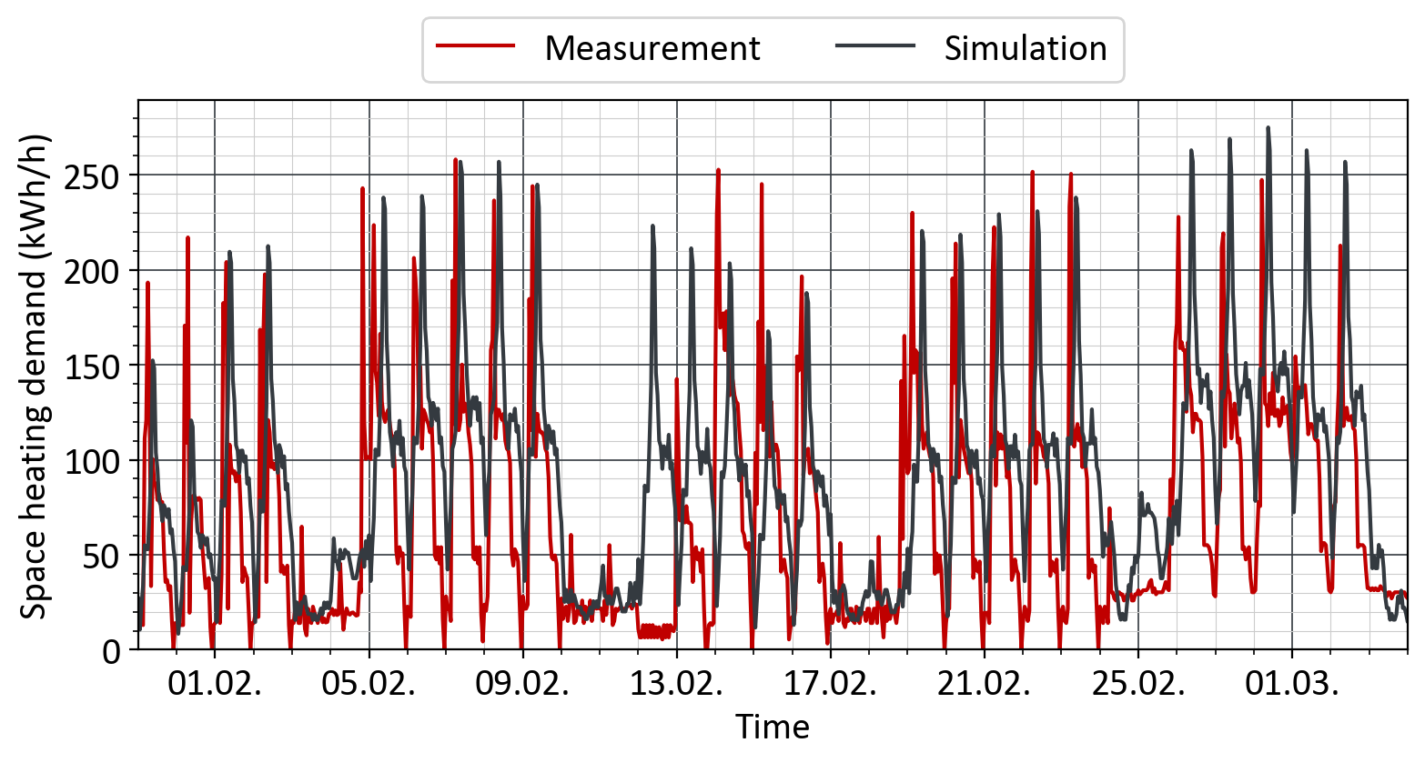
Figure 5 shows the heat demand profile of a secondary school (Aretzstraße 10, 52070 Aachen, Germany) for the period 14.3.-4.6.2018. Here, the transition from a cold period to a period of mild weather is shown. The week of 17.3. is still quite cold and a substantial heat demand occurs. The following week is significantly milder, which causes the heating demand to drop to almost zero. These effects can also be well represented by the simplified simulation procedure.
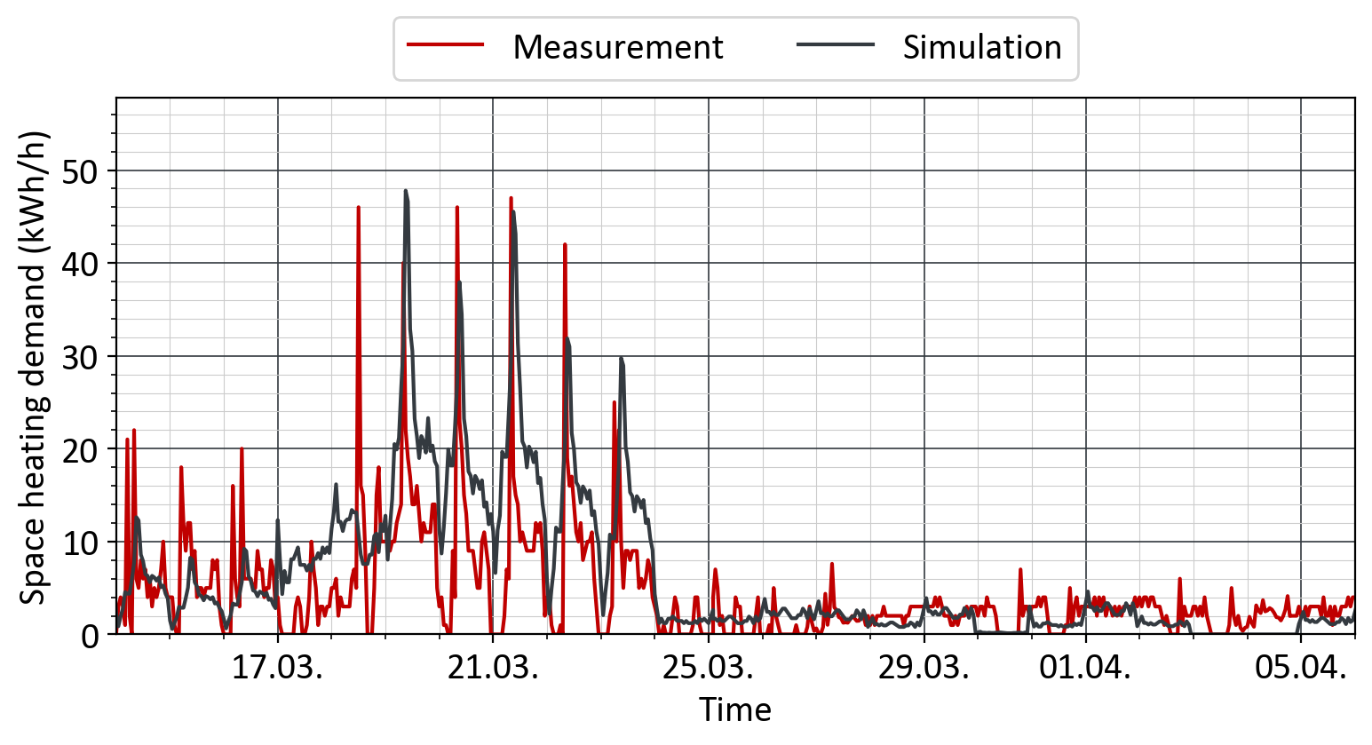
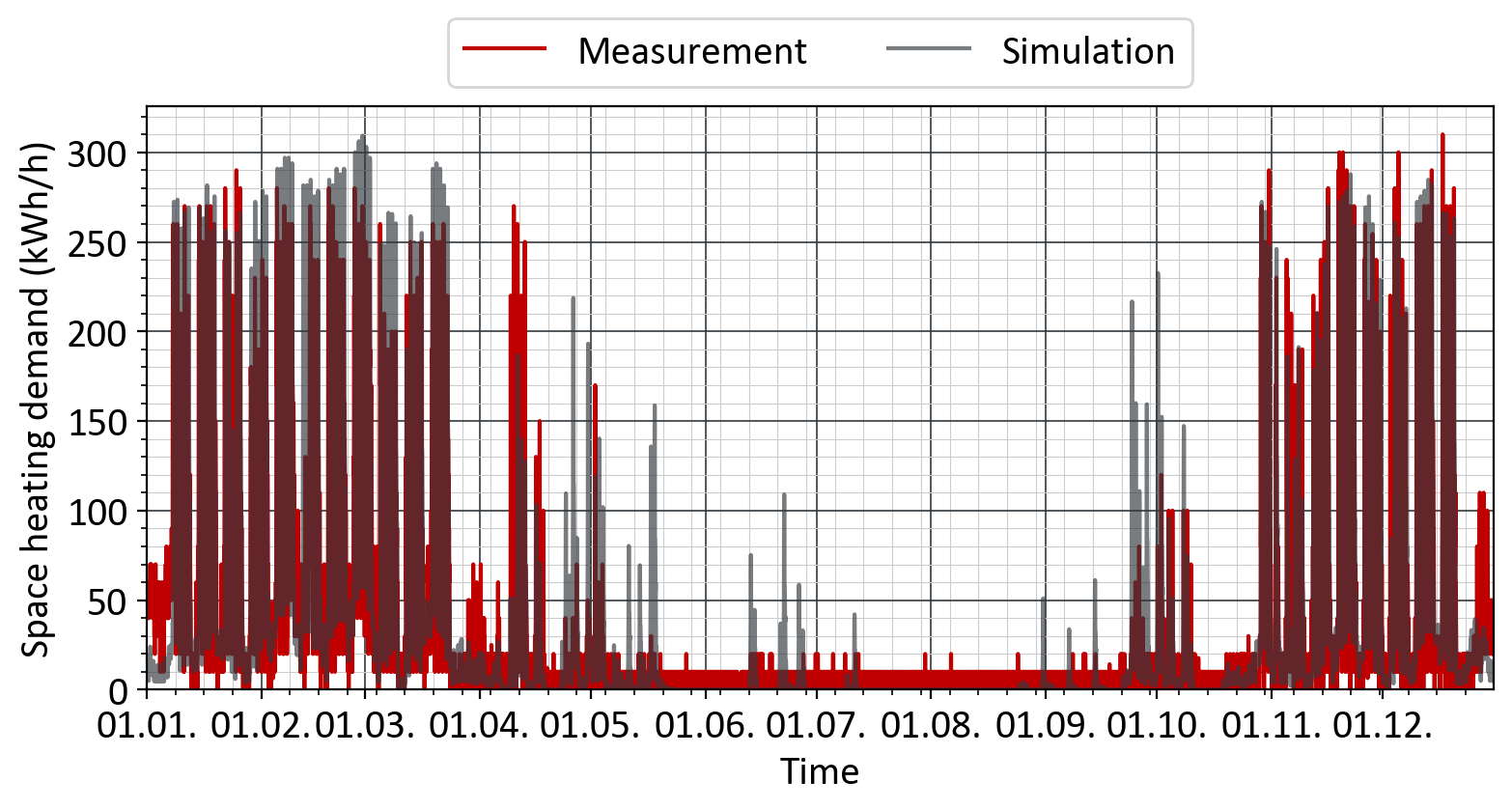
Figure 6 shows the heat load profile of a daycare center in Aachen for a whole year. It can be clearly seen that the heating phases in winter and the maximum heating load occurring there are well represented by the simulation. In summer, a low heat demand occurs in the measurement, which could be due to the domestic hot water preparation. The heat demand of the simulation drops to zero in summer since, in this case, the simulation only calculates the space heating demand.
 English
 Deutsch


